YAKCHDLRPBP stands for “Yet Another King County Housing Data Linear Regression Project Blog Post”.
Yep. That’s right. I just coined a new acronym.
But seriously, though, using the King County housing data set to build a Linear Regression project is so common these days that one can almost say, “if you’ve seen one then you’ve seen them all”.
Well, my hope is that my project stands out so that one can take away something new so that the above euphemism doesn’t apply.
You be the judge.
PROJECT OVERVIEW
Goals
Of course A goal in my project was to build a linear regression model that is statistically "reliable". But, for me, an even more important goal was to put that model to use to solve a hypothetical "real world" problem one might encounter when selling a home in King County. To that end, those goals were:- to provide an answer to the question, "which features can be FEASIBLY addressed by a seller to increase the sale price of his/her home?"
- to provide a CONCRETE strategy using an optimized linear regression model to accomplish this.
Approach
My high-level approach was to build the most “robust”, most predictive model - that is, with the highest Coefficient of Determination, \(R^2\), that reliably predicts our target, price, with minimized Root Moon Squared Error in the residuals - on the most optimal set of statistically significant features as possible.
High \(R^2\) is not enough!
We are not only interested simply in a high value in the the model’s Coefficient of Determination, \(R^2\), but we also want a good feel for the confidence of that measure.
"Overfitting" must be minimized
As part of the procedure when building the final linear regression model, I minimize overfitting with the use of *cross-validation* and combinatorics.
Data Bias must be minimized as much as possible
I employ the standard hold-out set technique to separate data when building models into the usual 0.70/0.30 split ratio of training data to testing data sets. Models are built using training data. Part of stastical “reliability” is achieved targeting models with the minimal \(\Delta RMSE\) between the predicted target (price) values from the training data set vs. the actual target values from the hold-out testing data set.
Model validation, Multicollinearity, and Feature Selection
Confidence in the computed Coefficient of Determination, \(R^2\), itself must be “measured” since not all \(R^2\)’s that are equal are created “equally” given the possibility for collinearity as well as “over-fitness”! These facets, if not addressed, will render a linear regression model stastically unreliable.In order to produce a model in which we can be confident in \(R^2\), I validate it deterministically.
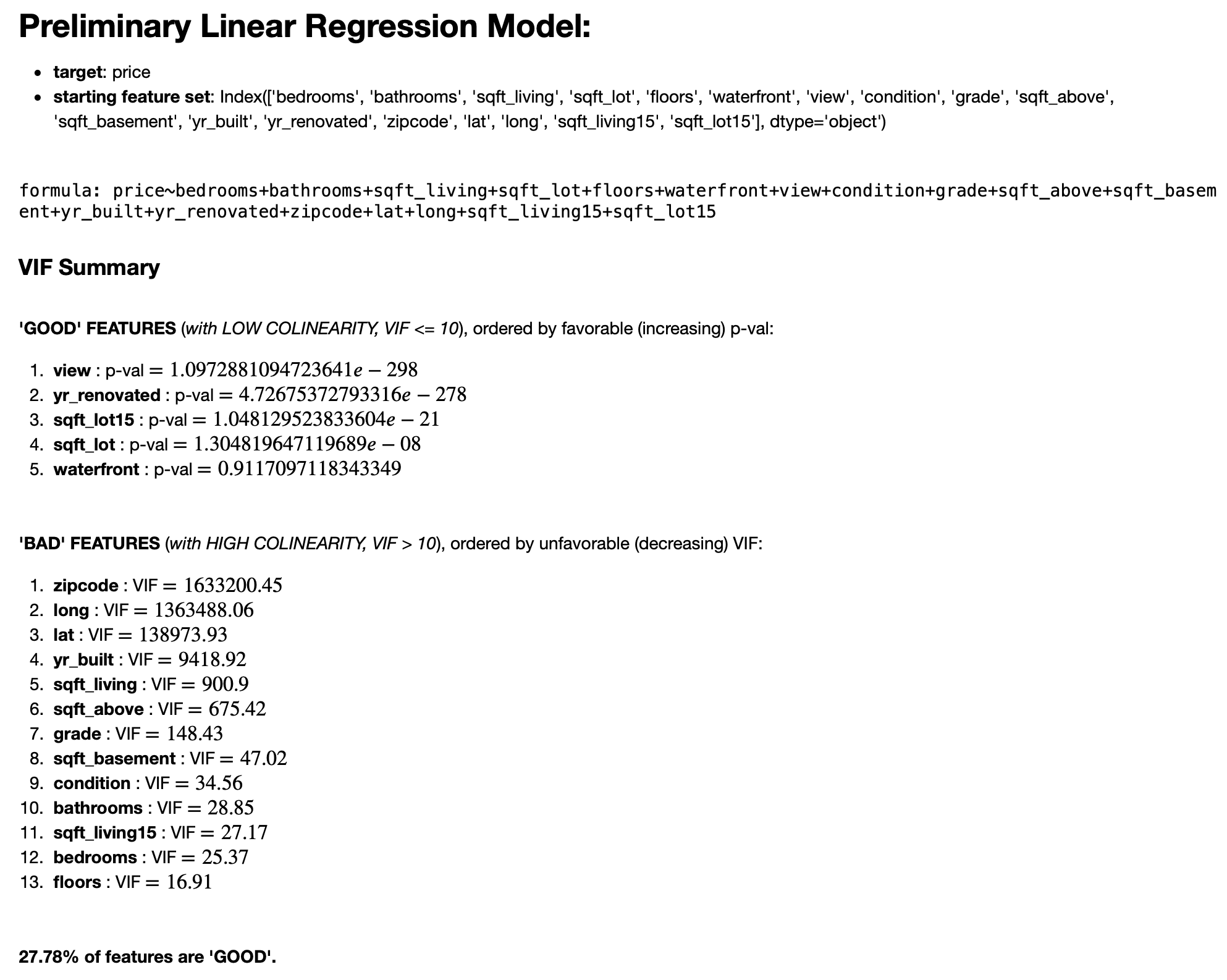
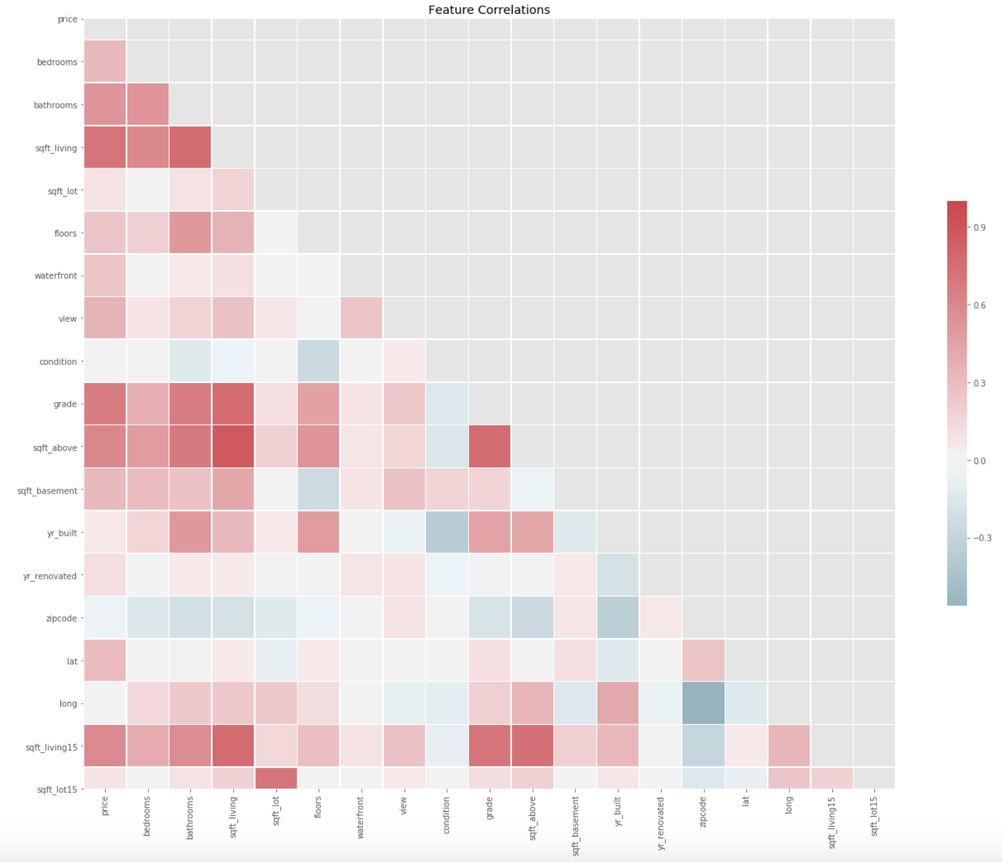
As will be shown, multicollinearity is a problem. When multicollinearity is present in a model, we cannot be confident in the statistical significance (p-value) of a collinear predictor. So, collinear predictors must be identified and dealt with in order to provide confidence in the measure of \(R^2\) and stastical signficance, in general.
There are two means of handling collinearity of predictors:
- Introduce an interaction term, which will effectively combine two collinear predictors in the model, or
- Drop a term (feature) from a given set of collinear predictors.
Either approach taken must be backed by mathematical rationale. That is, some mathematically deterministic method must be employed to first *select* (identify) which features are collinear.
But, I take the latter approach.
Variance Inflation Factor
According to James, Witten, Hastie & Tibshirani, a ... way to assess multi-collinearity is to compute the variance inflation factor (VIF). The VIF is the ratio of the variance of [the coefficient of a predictor] when fitting the full model divided by the variance of [the coefficient of a predictor] if fit on its own. The smallest possible value for VIF is 1, which indicates the complete absence of collinearity. Typically in practice there is a small amount of collinearity among the predictors. As a rule of thumb, a VIF value that exceeds 5 or 10 indicates a problematic amount of collinearity.(James, Witten, Hastie & Tibshirani, 2012)
Exploratory Data Analysis and Regression Diagnostics
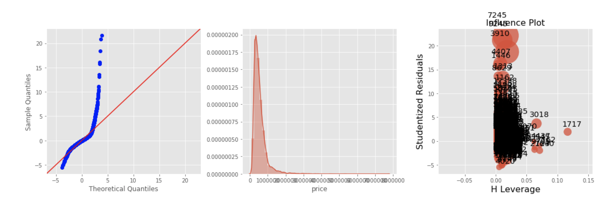
Utilizing Regression Diagnostics is a key part of the Exploratory Data Analysis phase. A primary output of this phase is to produce a cleaned data set in which outlier and null values have been “dealt with”. Additionally, Regression Diagnostics, via visualization, provide some insight into the distributions and kurtosis of predictors, as they relate to the target response variable. Regression Diagnostics are, therefore, utilized to provide insight into whether or not predictors must be transformed.
Forward Selection of Features
Rather than making “educated guesses” in the feature selection process, after cleaning the data set, I use cross-validation, k-folds, and combinatorics to select the “best” model (from the best feature-set combination) built on training data when compared to testing data, based a simple, greedy forward selection using dynamic programming. I authored another blog post focusing specifically on the algorithm I wrote to accomplish this task. But, some effort is made up front to “intelligently” reduce the set of starting features by building a preliminary model and then removing features which obviously do not inluence price or are highly correlated, based on Regression Diagnostics as well as the Variance Inflation Factor (VIF) of a given feature.
Conditions for success - i.e. whether a linear regression model is "good" or "bad"
Given the following conditions, we have a “GOOD” model when:1. \(R^2 > .60\)
2. \(|RMSE(test) - RMSE(train)| \approx 0\)
3. low Condition Number (measure of collinearity)… much less than 1000; but I target Condtion Number threshold of 100 or less
The first condition says that we want models that determine the target with greater than 60% “confidence”.
The second condition says that the bias toward the training data is minimal when compared to how the model performs on the “hold-out” test data.
The third condition requires that collinearity be mitigated/minimized.
Toward Regression: Most important aspect is understanding the data!
To that end, I follow the standard OSEMN model (Lau, 2019) and proceed according to the following steps:- Import all necessary libraries and the the data set
- Cleaning the data set:
- Clean null values, if any
- Clean outlier values, if any
- Convert feature data types as necessary
- EDA: Gain familiarity with the data set by building a preliminary linear regression model
- Utilize Regression Diagnostics: using Regression Diagnostics is of fundamental importance since it will provide some guidance on whether or not a feature should be transformed
- Explore distriubutions
- Explore collinearity
- EDA: Scale, Normalize, Transform features in the data set as necessary for the working model
Build the "Optimal" Model
After the data is cleaned and all of the required transformations exexuted on the predictors, and after having initially "weeded out" predictors which do not manifest a linear relaltionship to the target response variable, I execute the above-mentioned algorithm to select the set of features which will result in the optimal model according to the criteria mentioned in the "Conditions for Success" section. At this point, I will have the optimal model for this data set that is statistically "reliable".
Run linear regression experiments to answer real questions
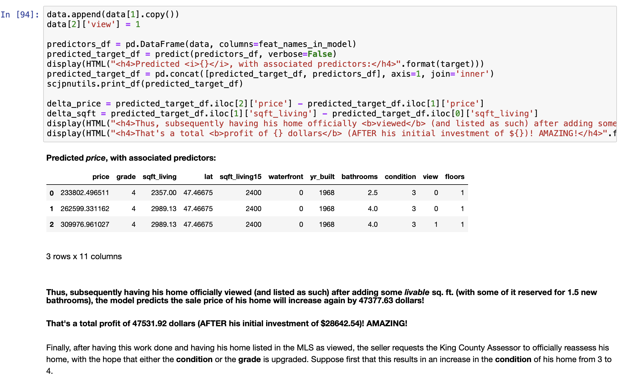
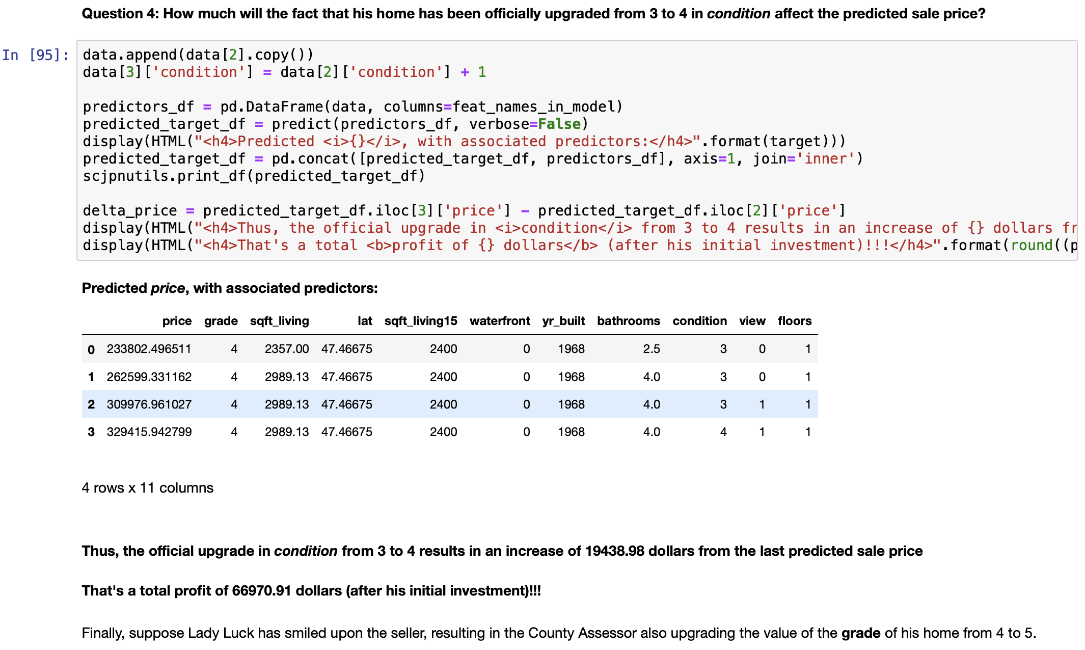
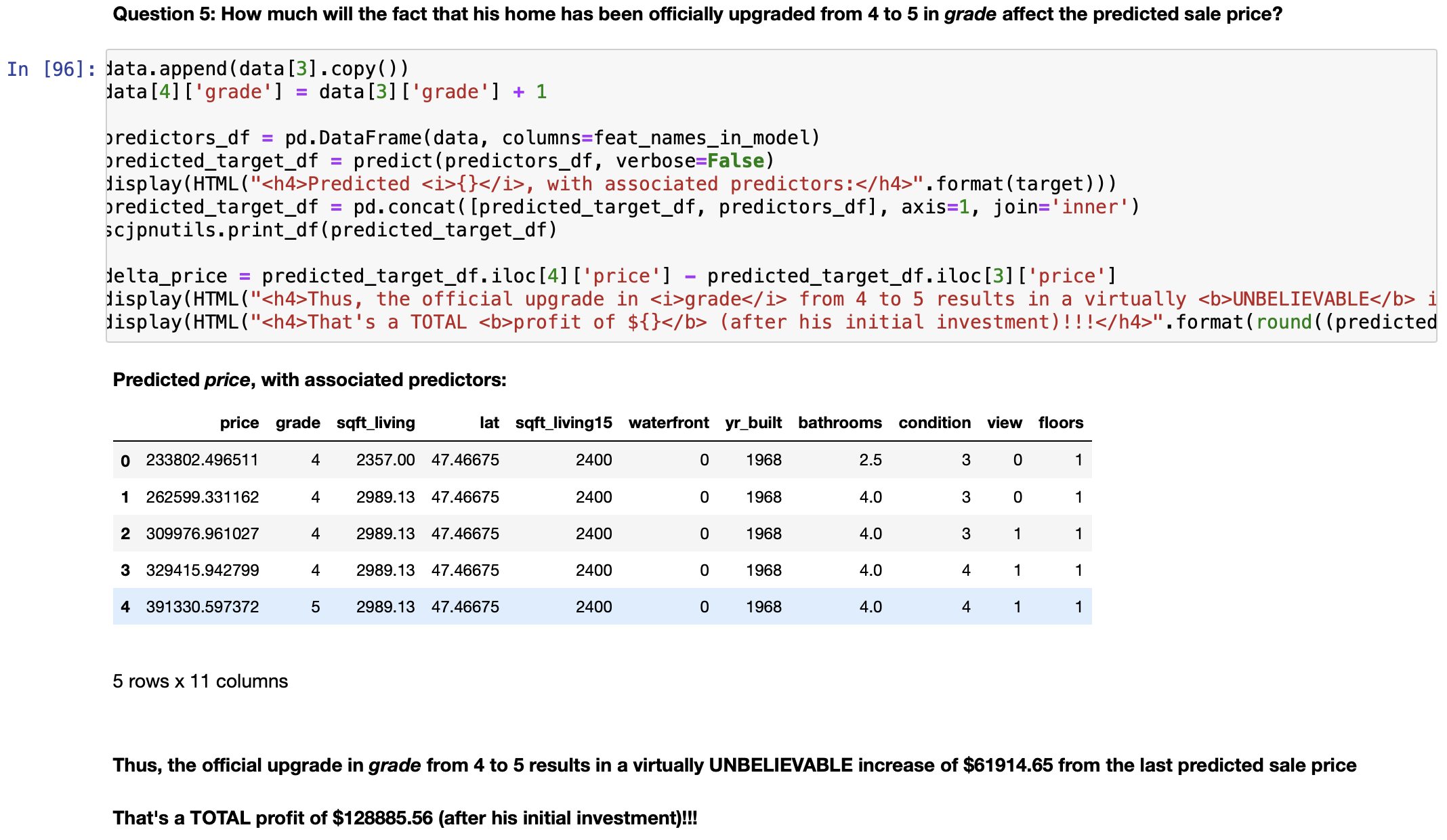
Now this is arguably the "funnest" phase of the project.With the optimal model in hand, I attempt to apply it toward a hypothetical "real world" problem:
- Which features can be feasibly addressed by a seller to increase the sale price of his/her home?
- Provide a concrete strategy using the optimized linear regression model to accomplish this.
THE PROCESS
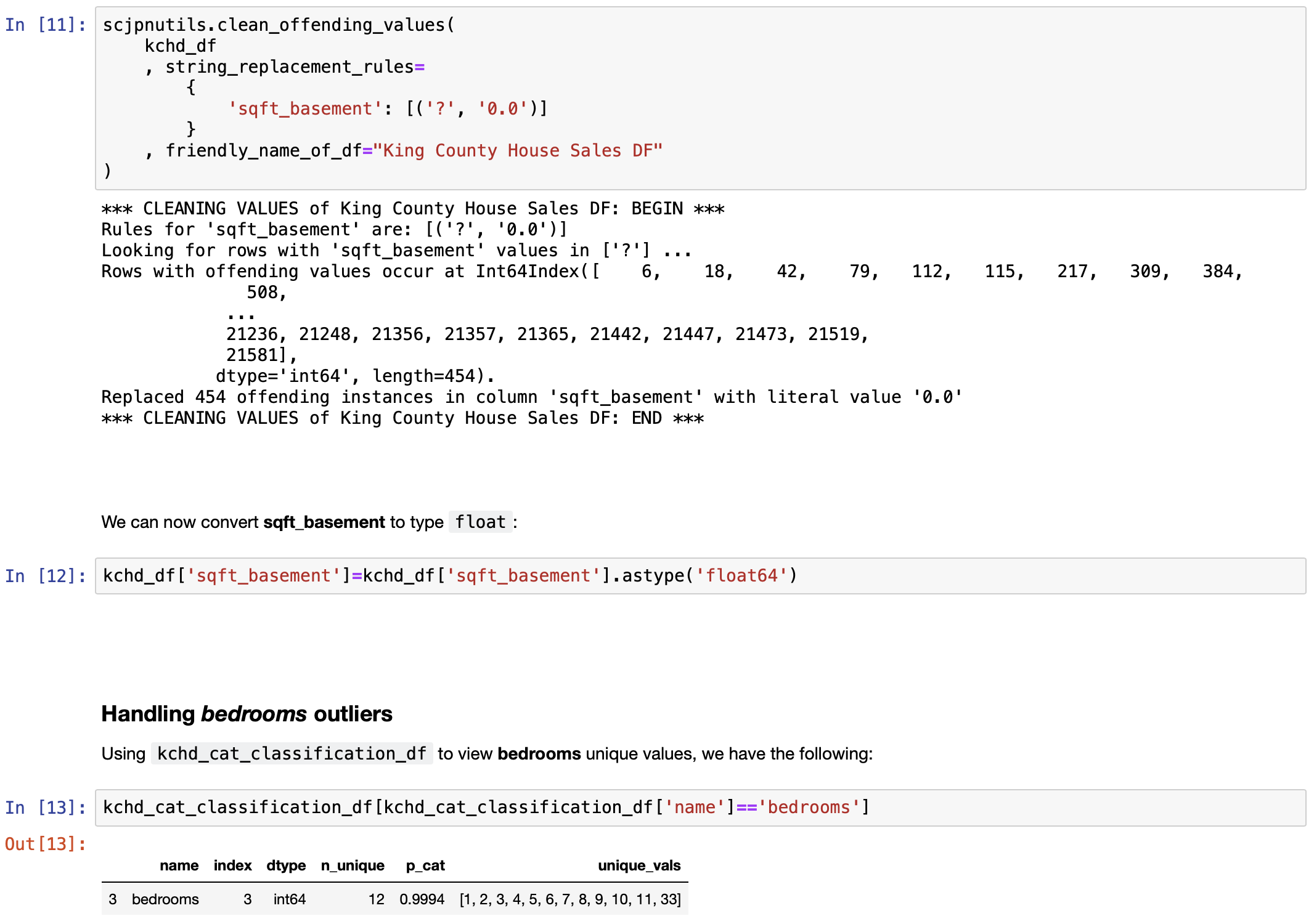
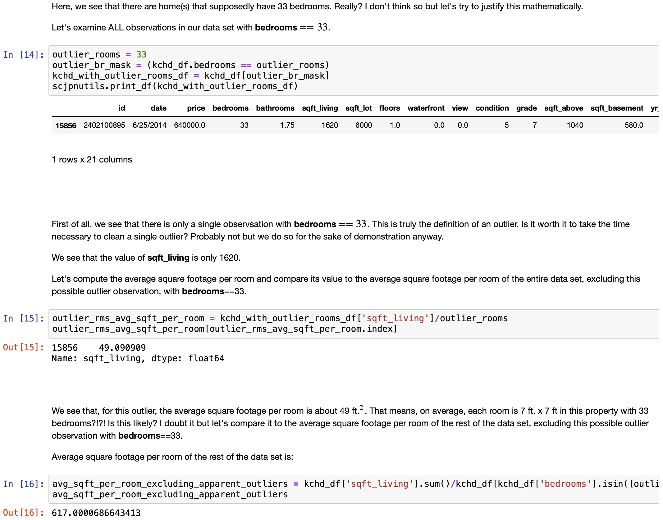
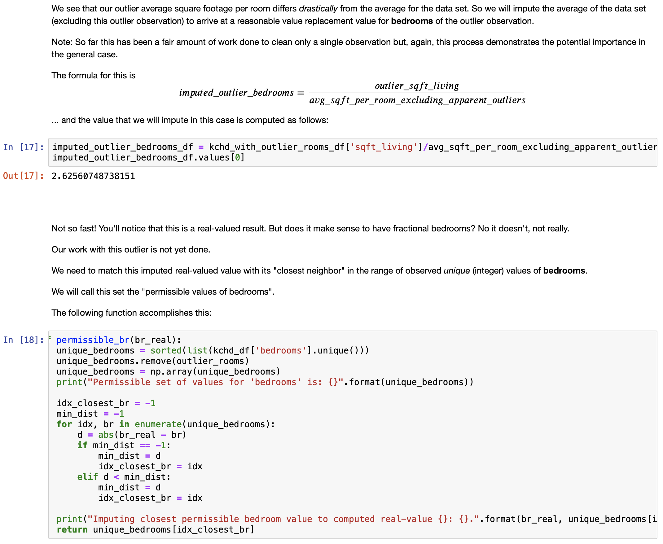
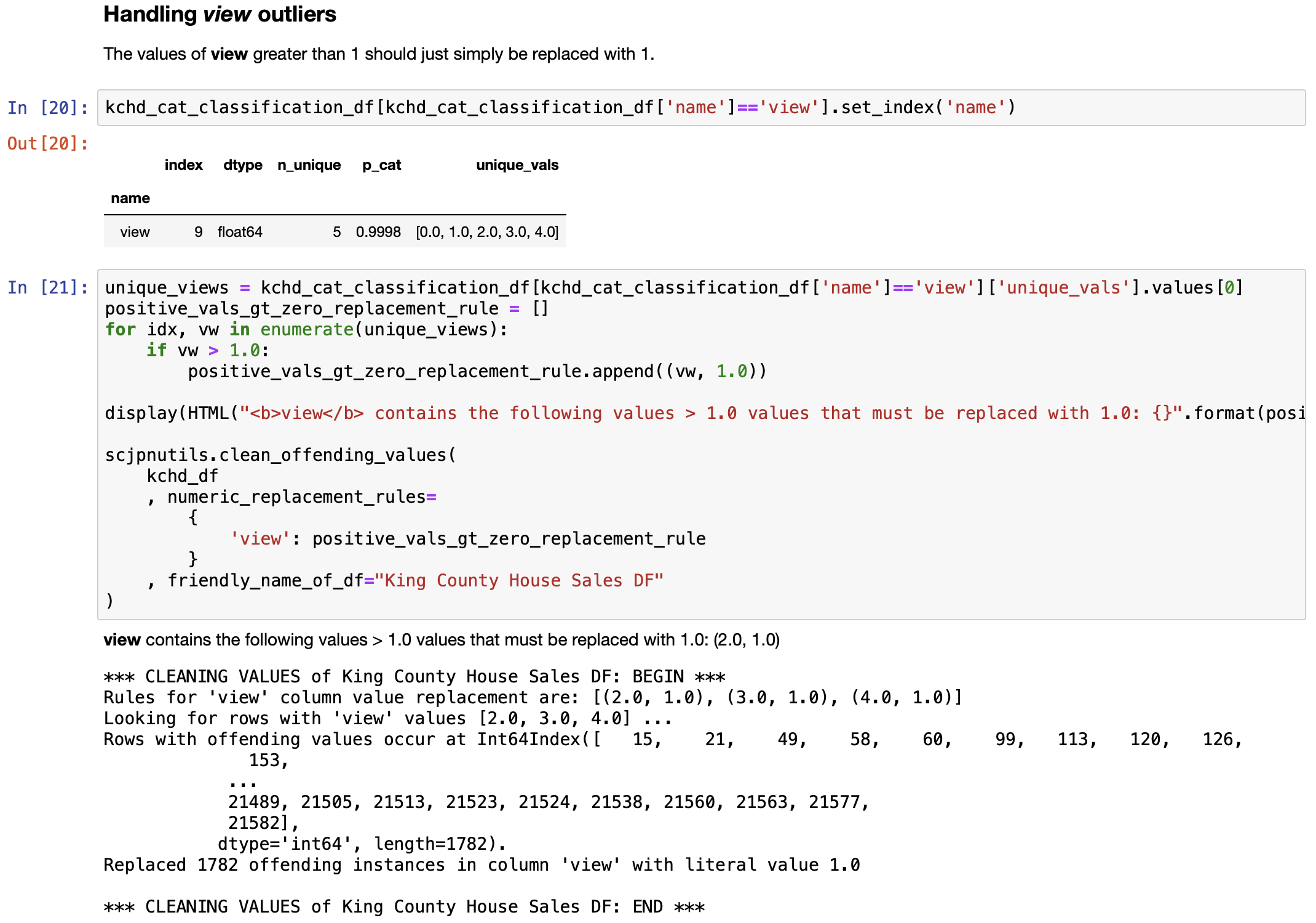
Cleaning the Data Set and EDA
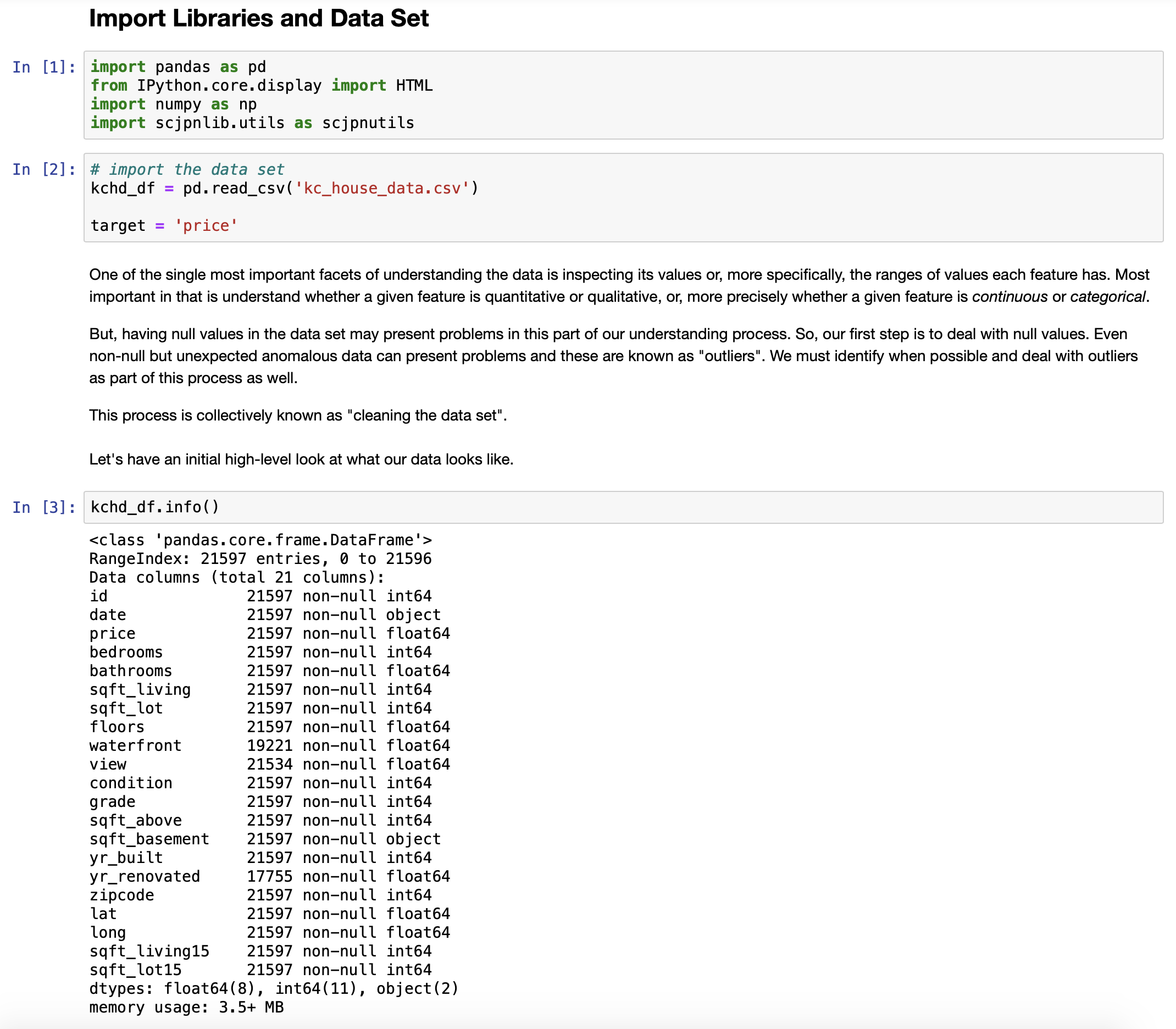
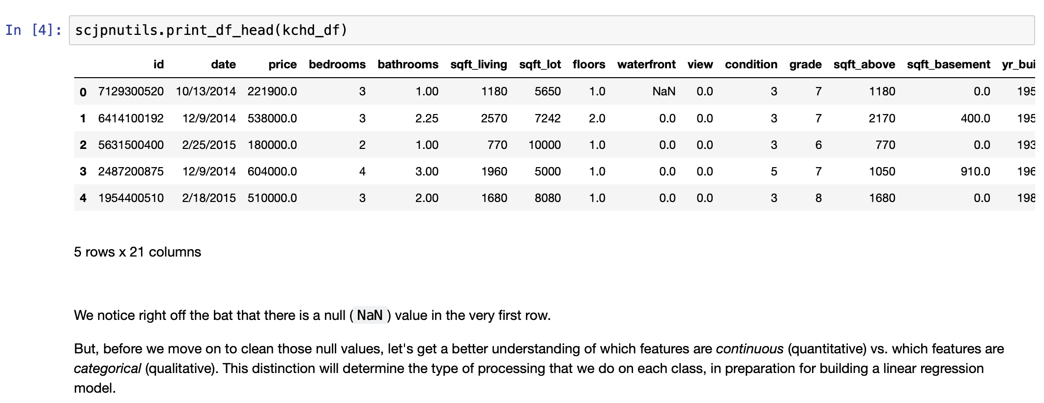
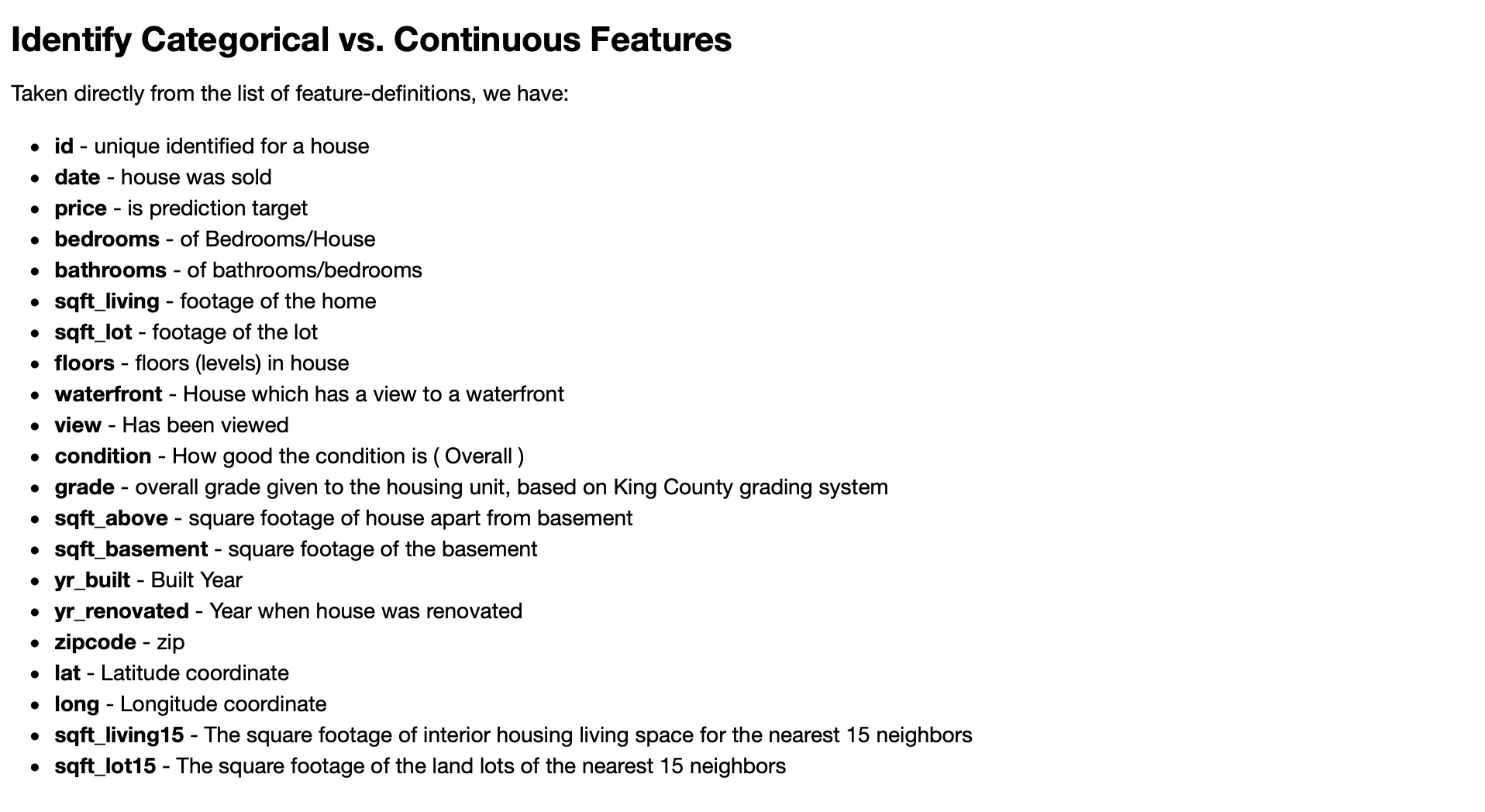
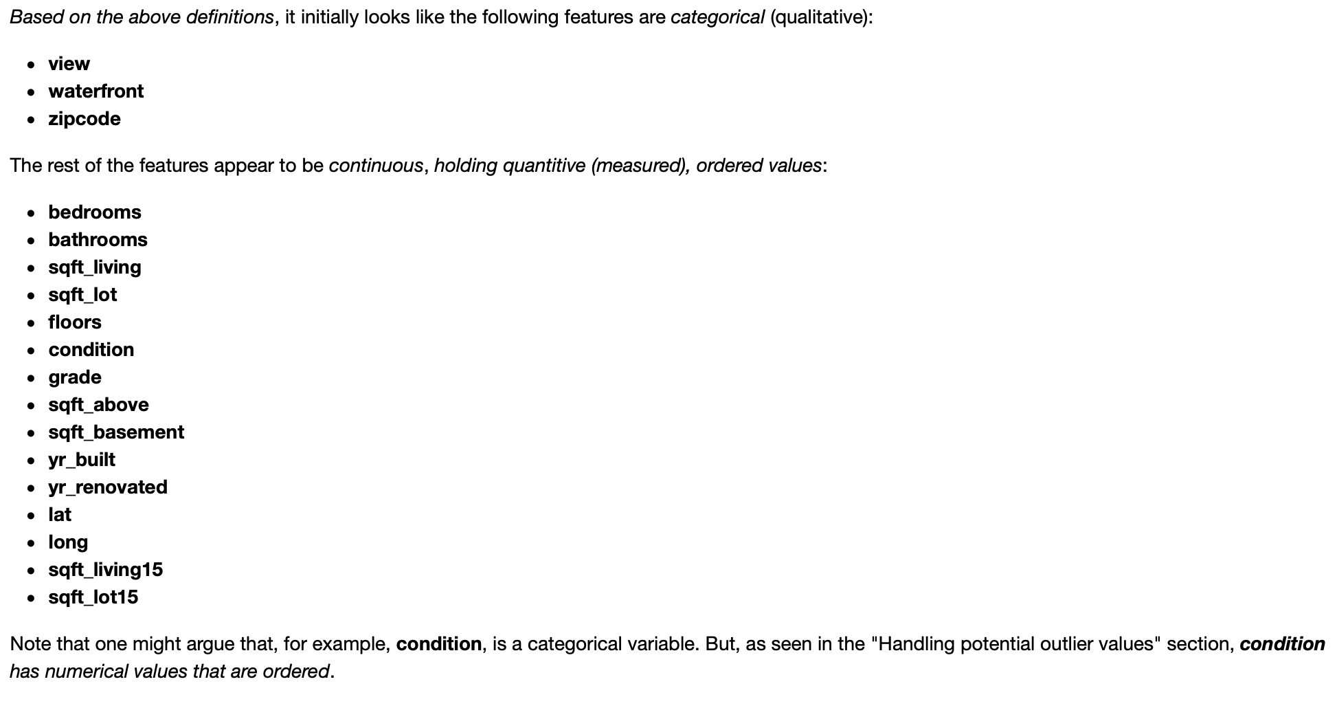

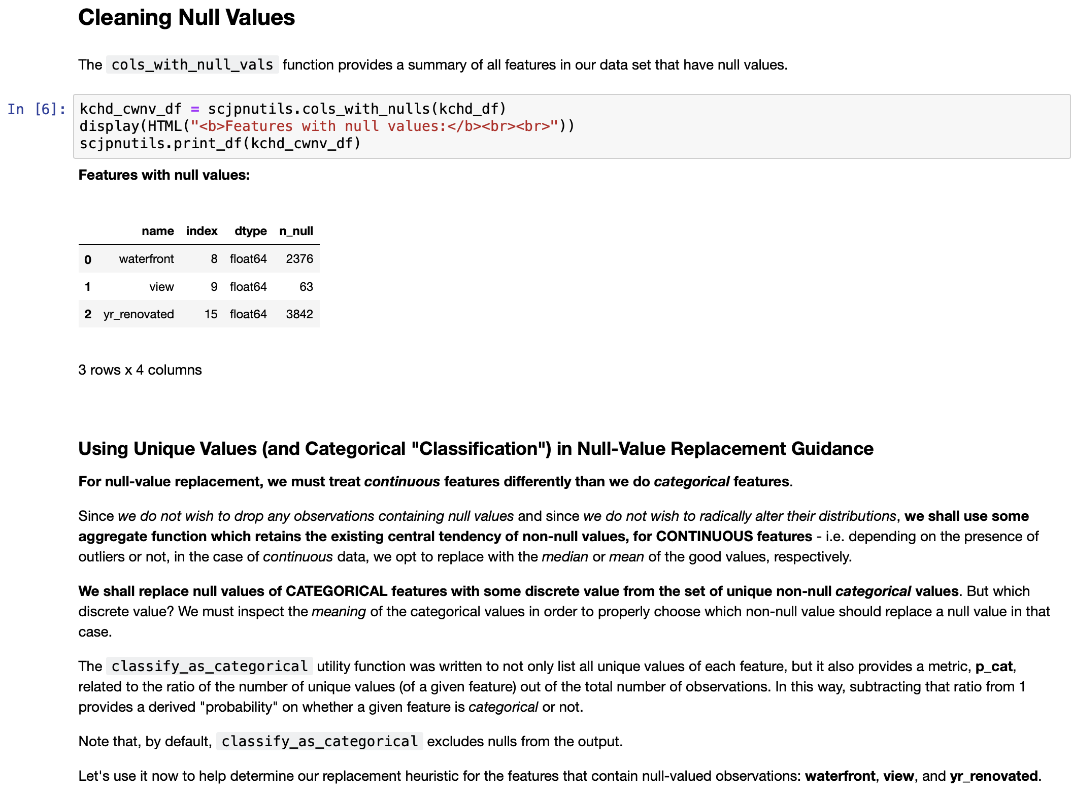
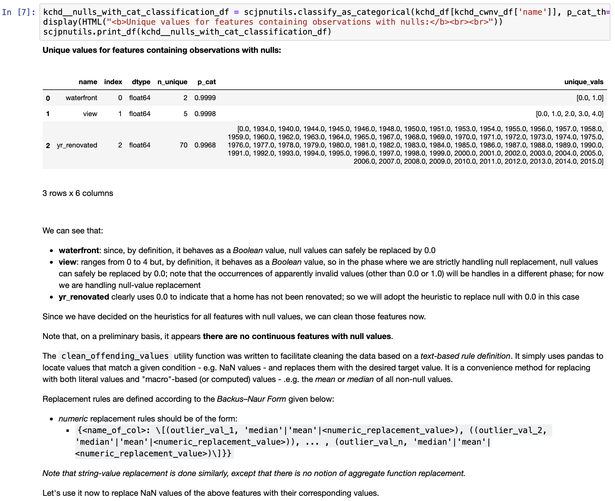
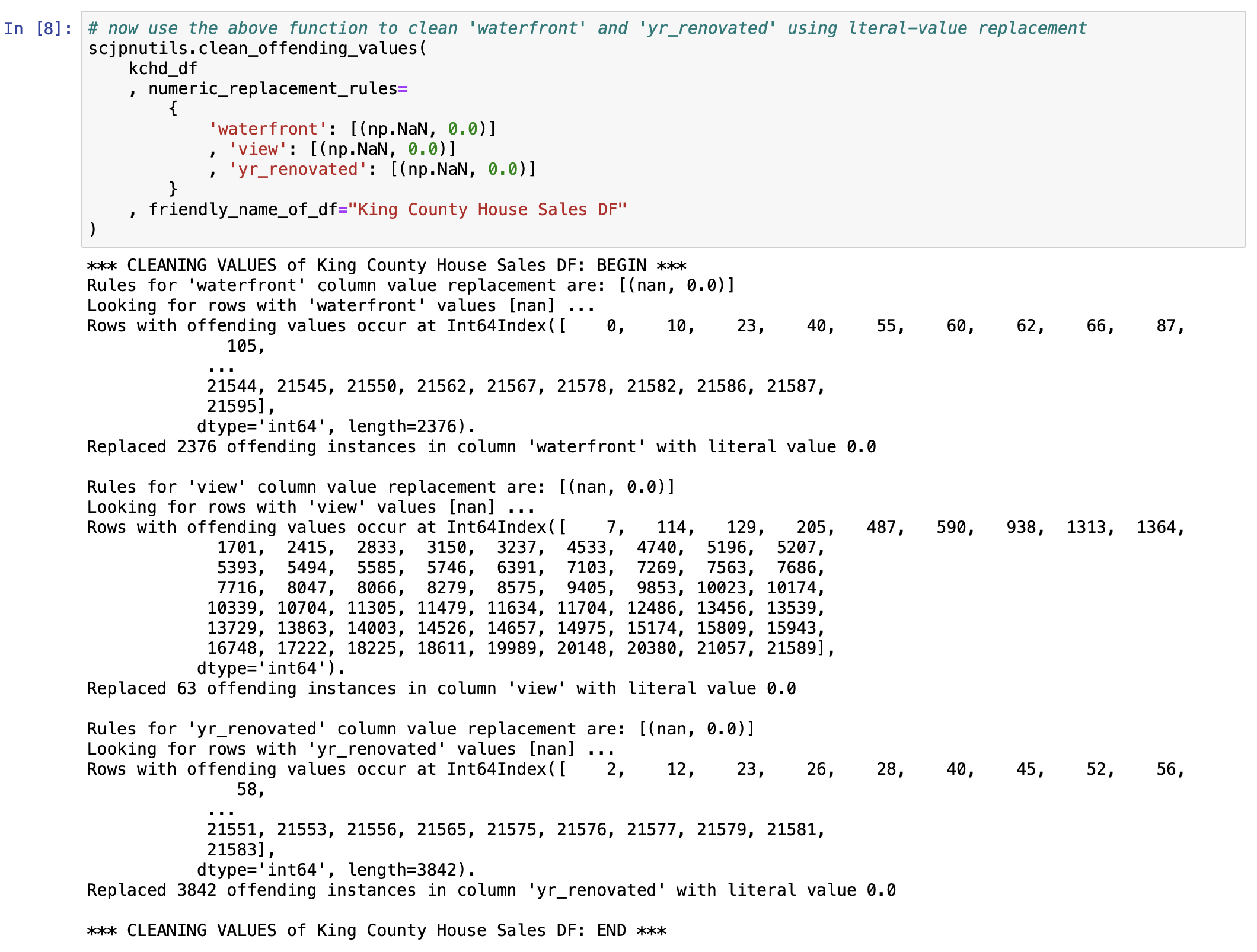


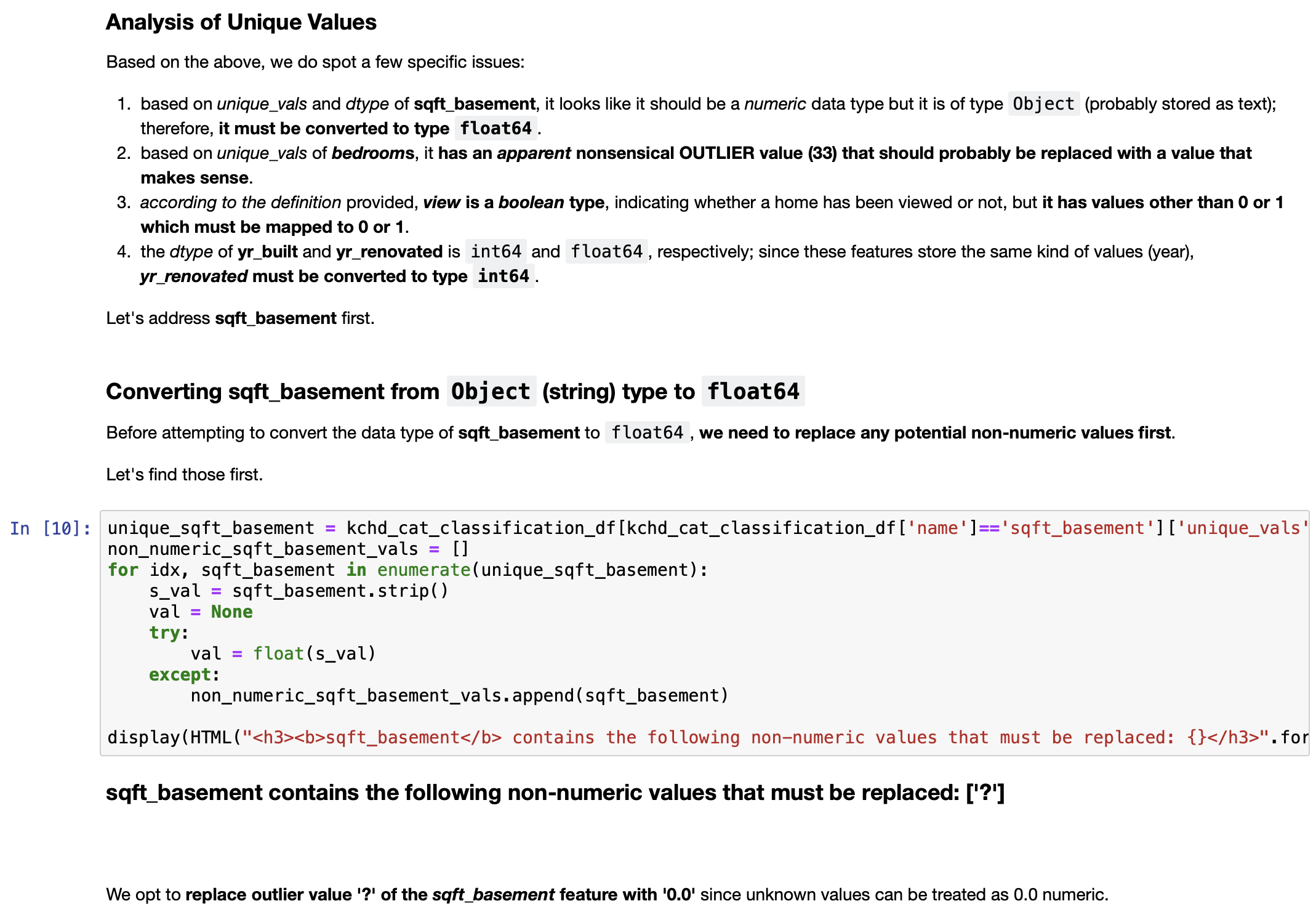
Note: output has been truncated in order to save space, therefore the list above is incomplete; for the full list, please refer to the Step 2 Jupyter notebook.



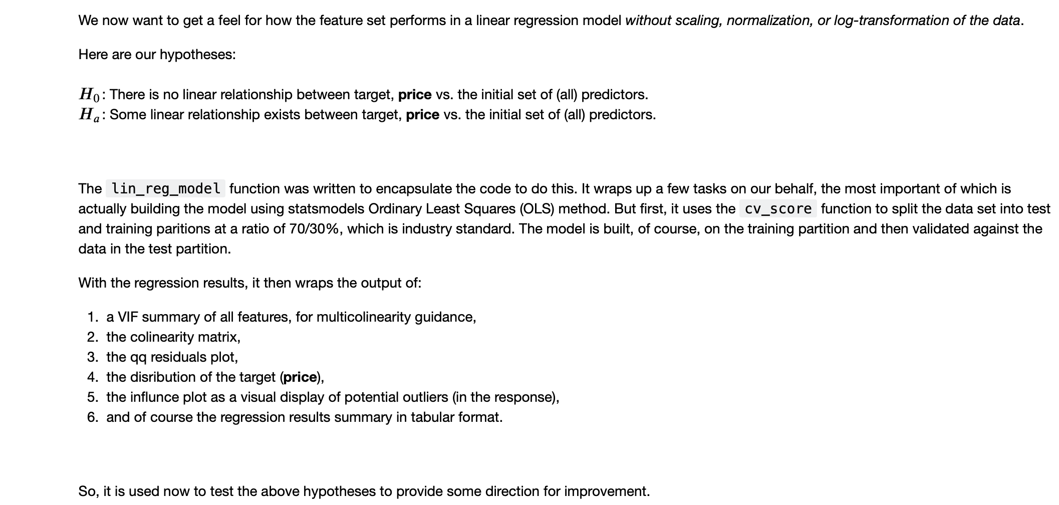
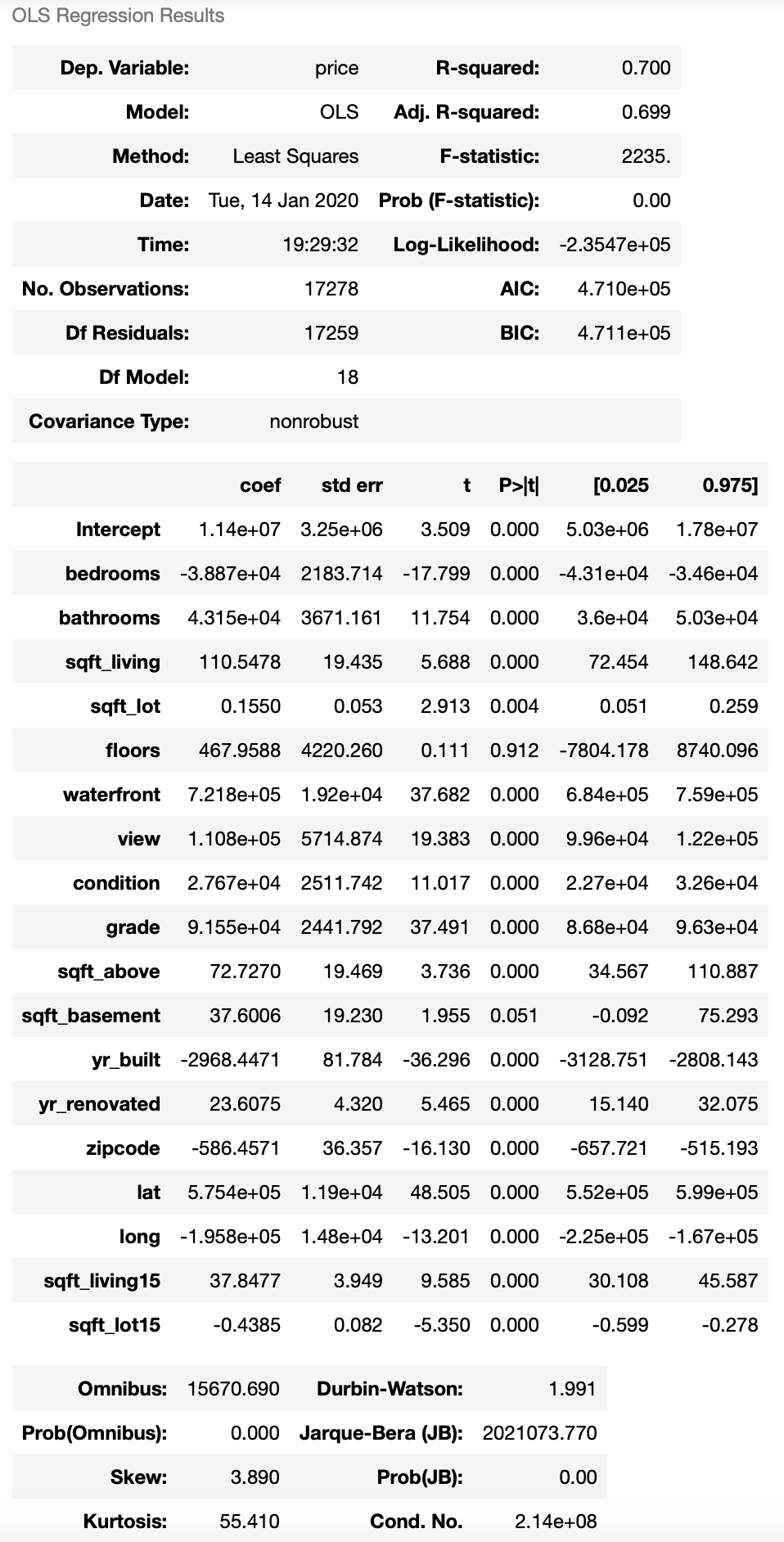
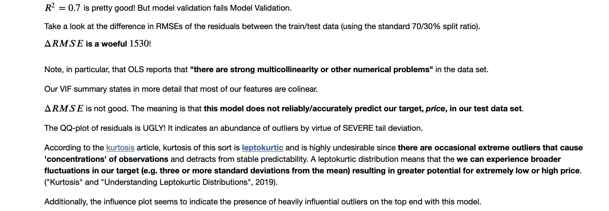
EDA: Getting to know the data via a Preliminary Linear Regression Model (based on the cleaned data set)



EDA: Iterative Model Refinement

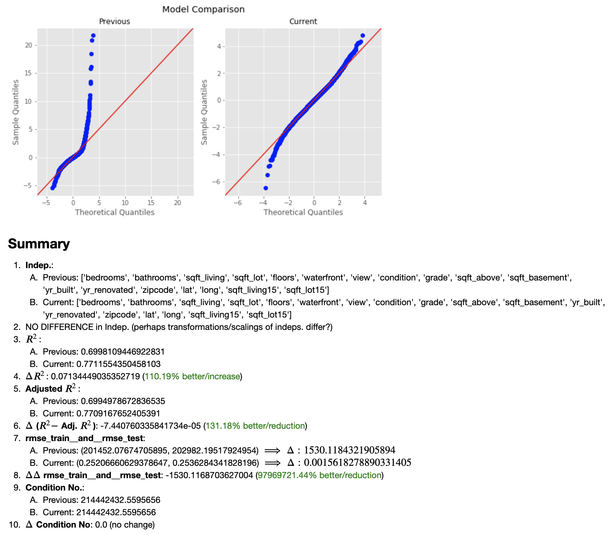
Note: output has been truncated in order to save space, therefore, I present only the resulting model comparison; for the full model output, please refer to the main notebook.
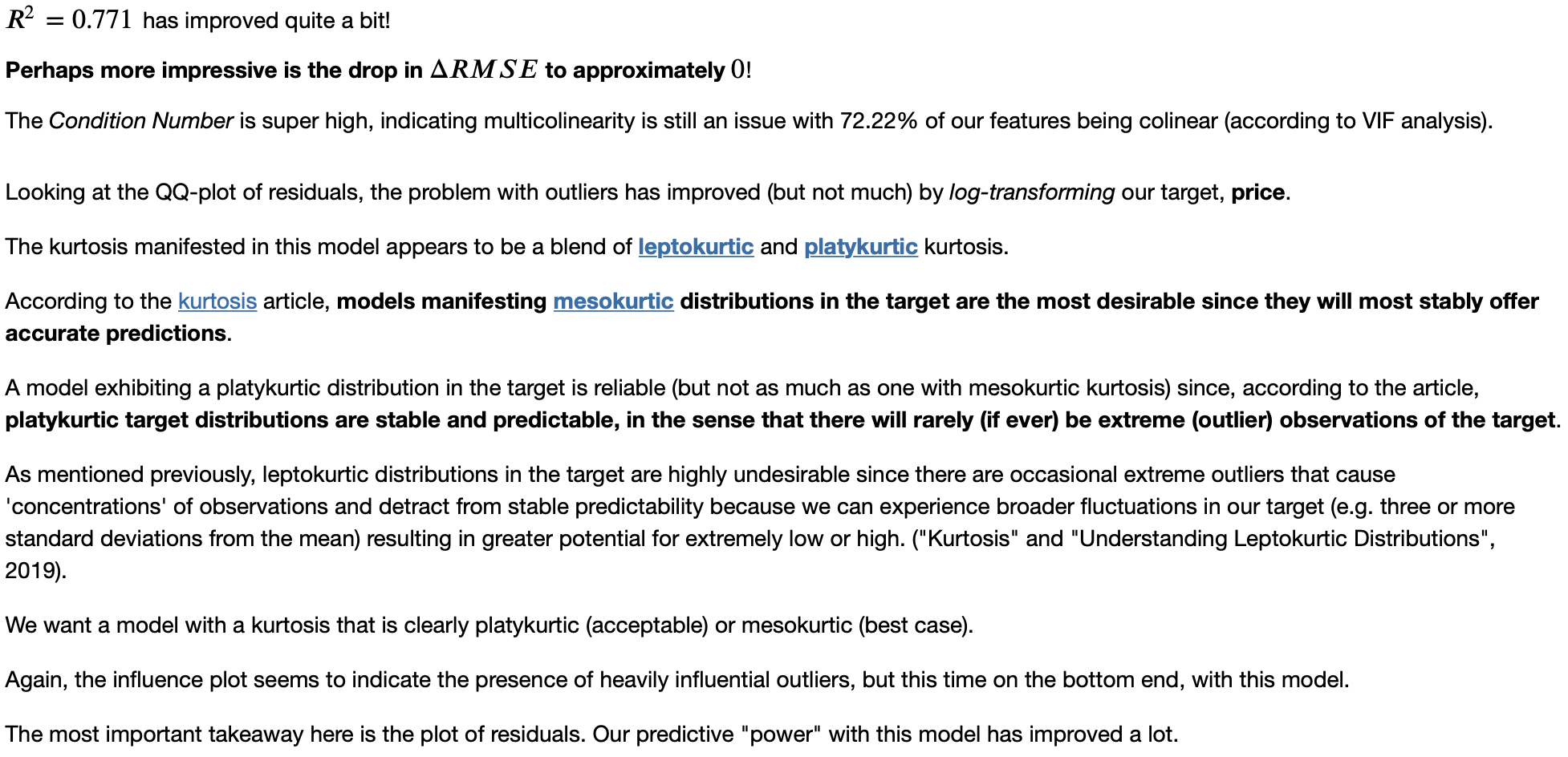

Regression Diagnositcs: A Deeper Feature Understanding and a Pathway to Feature Tuning

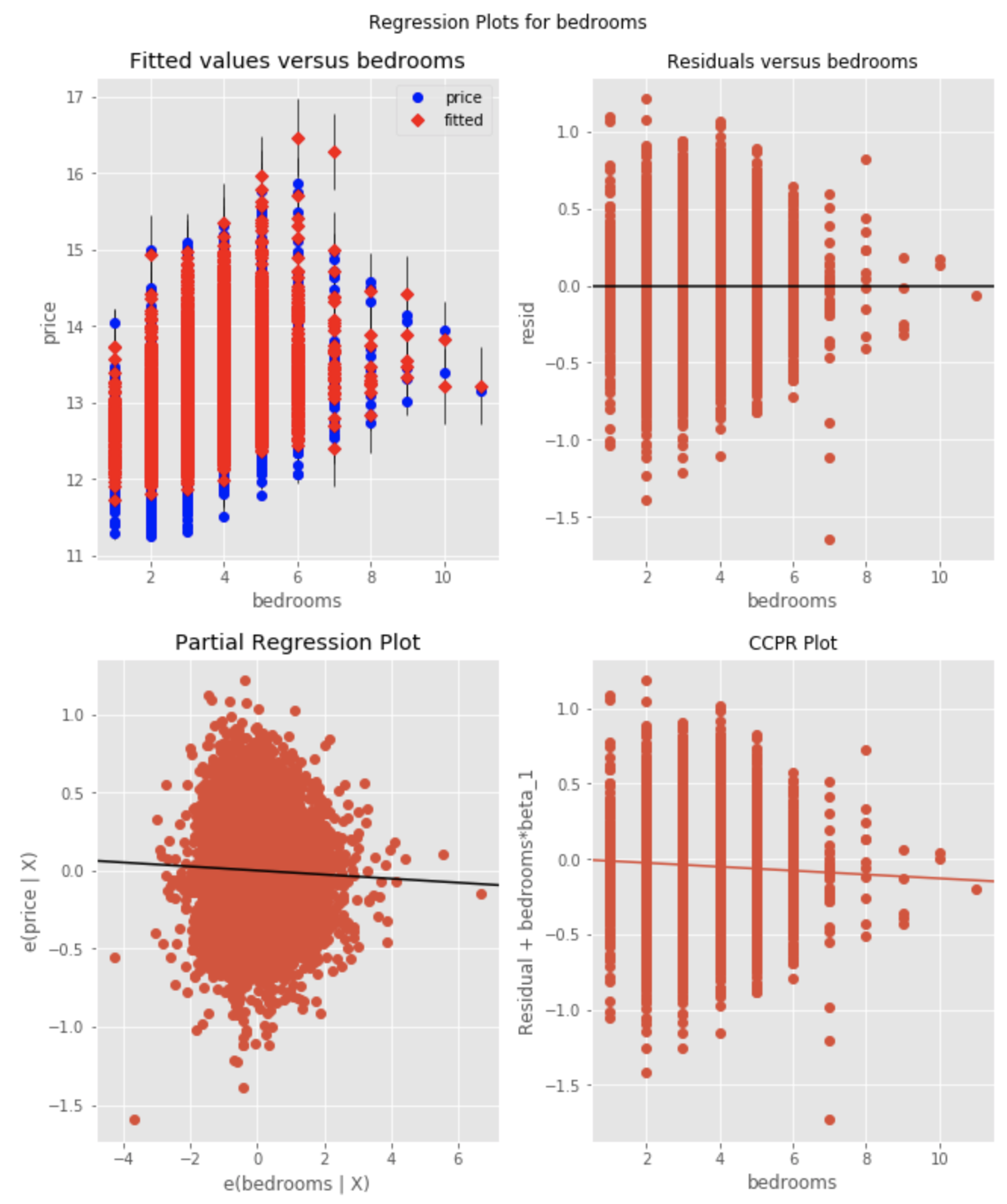
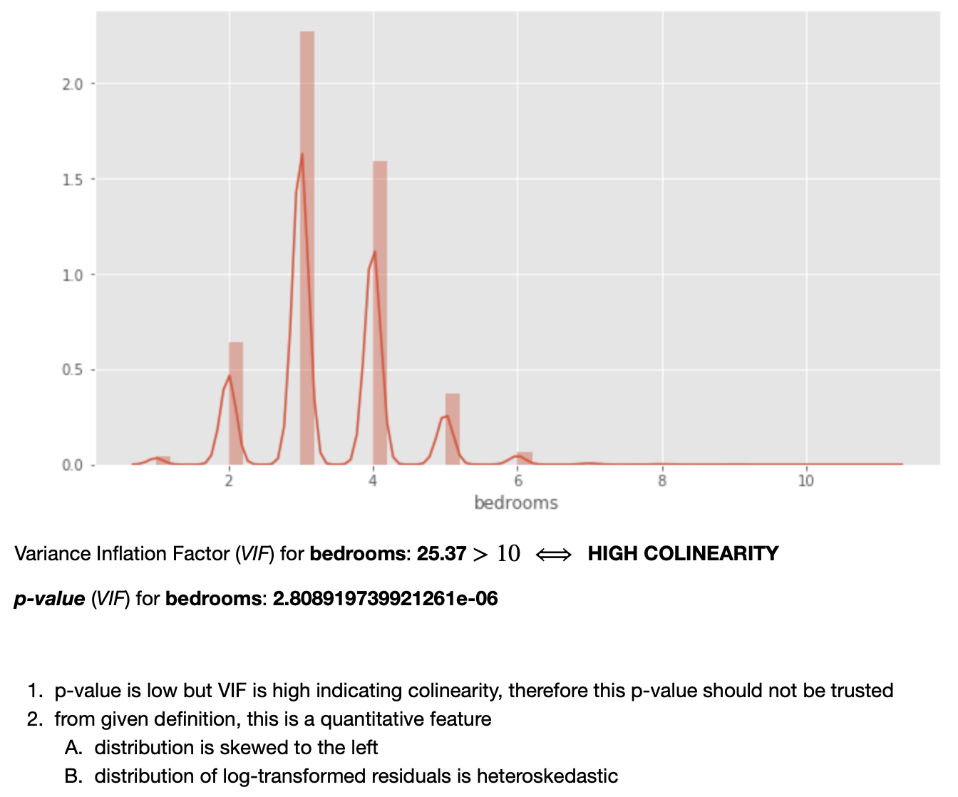
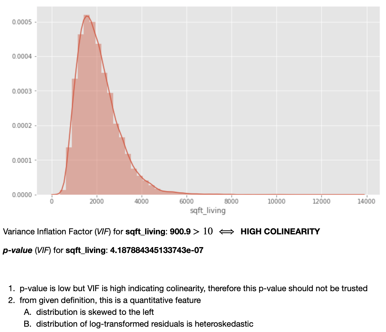
Note: although it is not stated in "plain English" in the notebook, the fact that the distrubtion of residuals is heteroskedastic (as well as the distribution of the predictor itself) suggests that this predictor ought to be transformed (log-transformed).

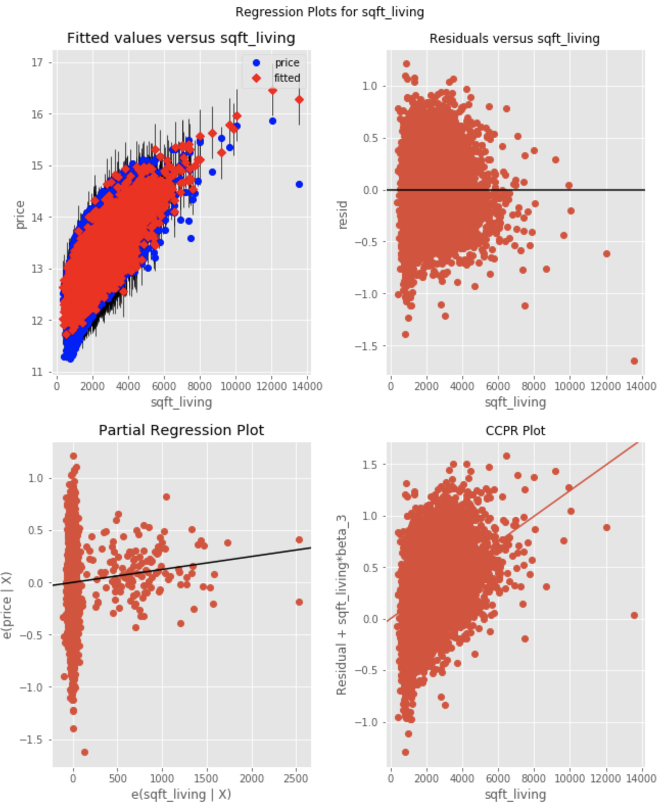

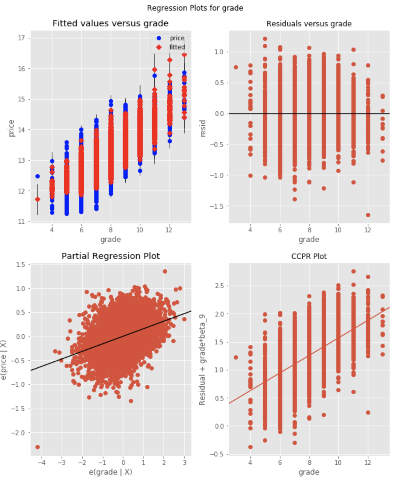
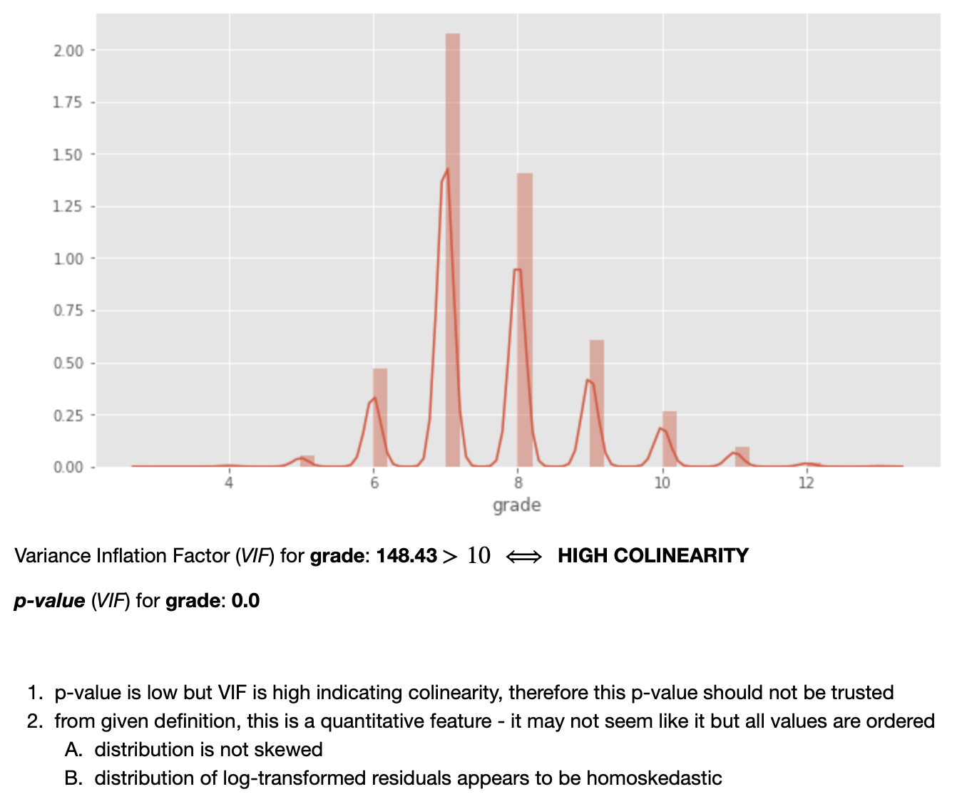
Note: although it is not stated in "plain English" in the notebook, the fact that the distrubtion of residuals is homoskedastic (as well as a relatively normal distribution of the predictor itself) suggests that this predictor should NOT be transformed (log-transformed); thus, it is simply tracked as a "normal" continuous variable (not to be transformed later).

Note: output has been truncated in order to save space but from here I follow the same pattern to complete this study of all of the predictors in the last model to get a clear idea of which ones should be transformed and which shouldn't; for the full output of Regression Diagnostics, please refer to the main notebook.
Feature Scaling/Normalization and Transformation: Put the insight garnered from the Analysis of Regression Diagnostics to use!

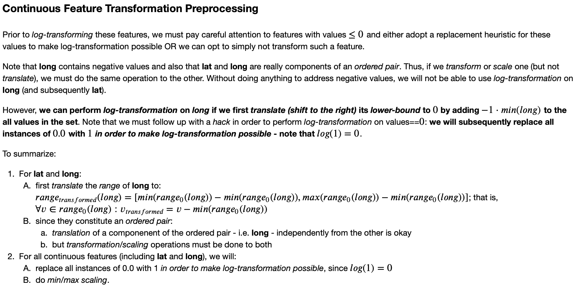

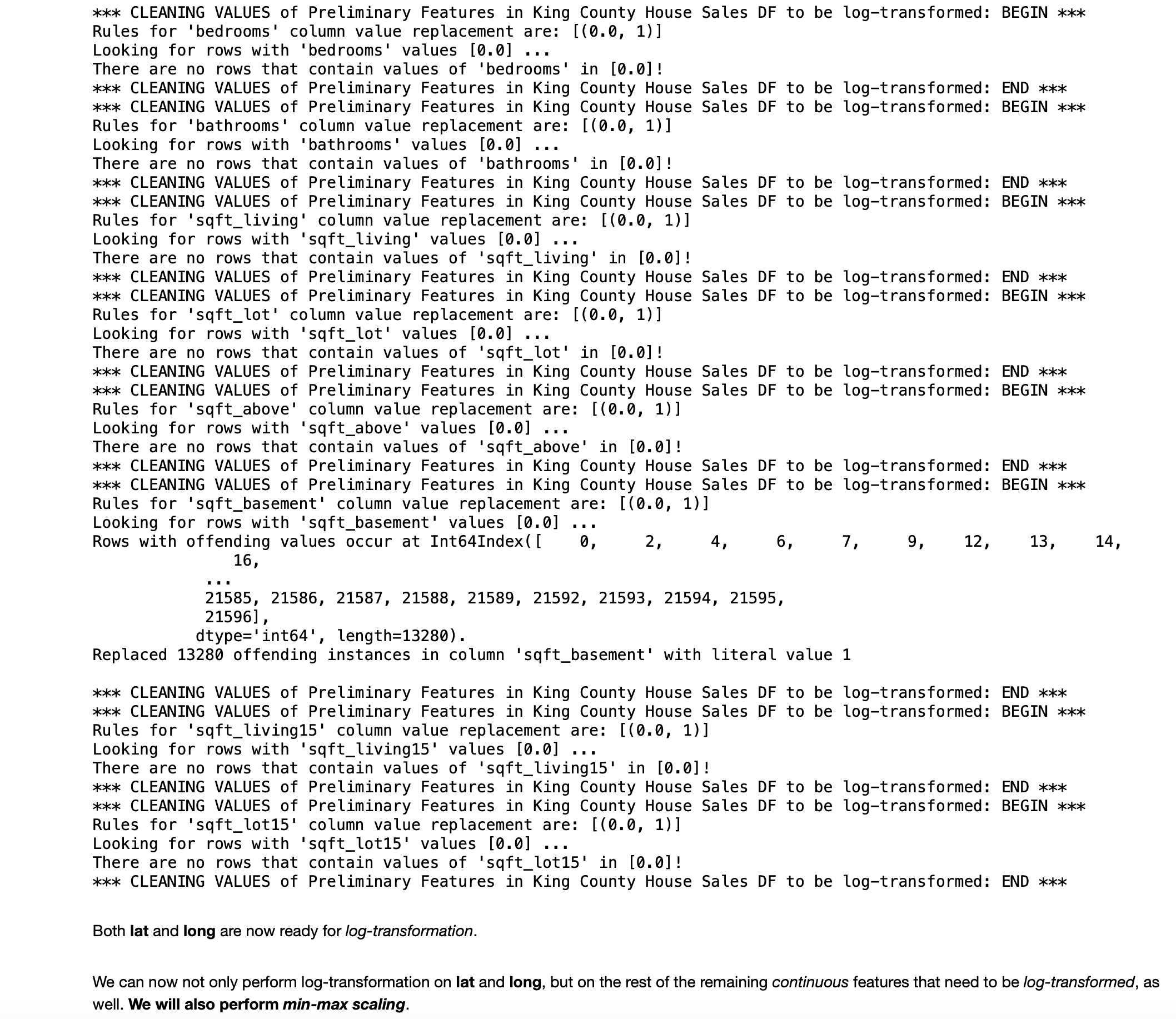
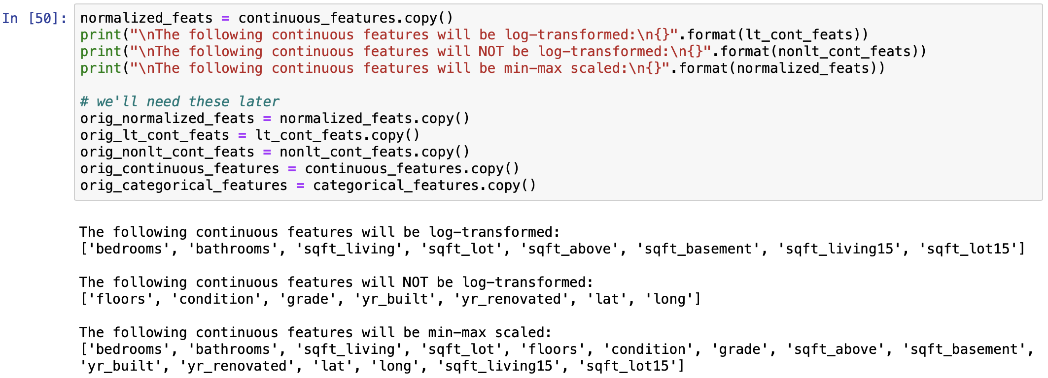
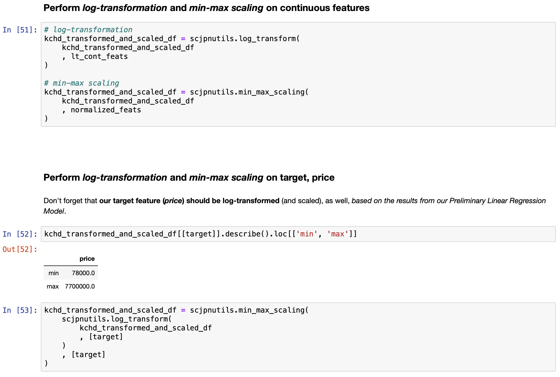

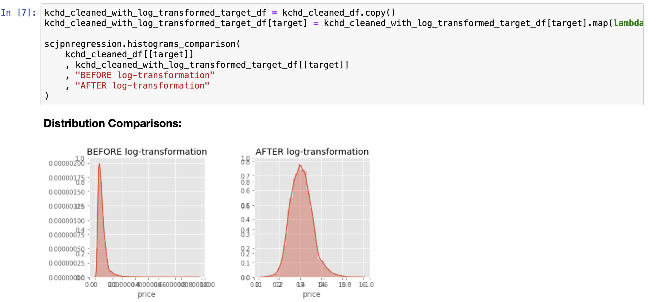
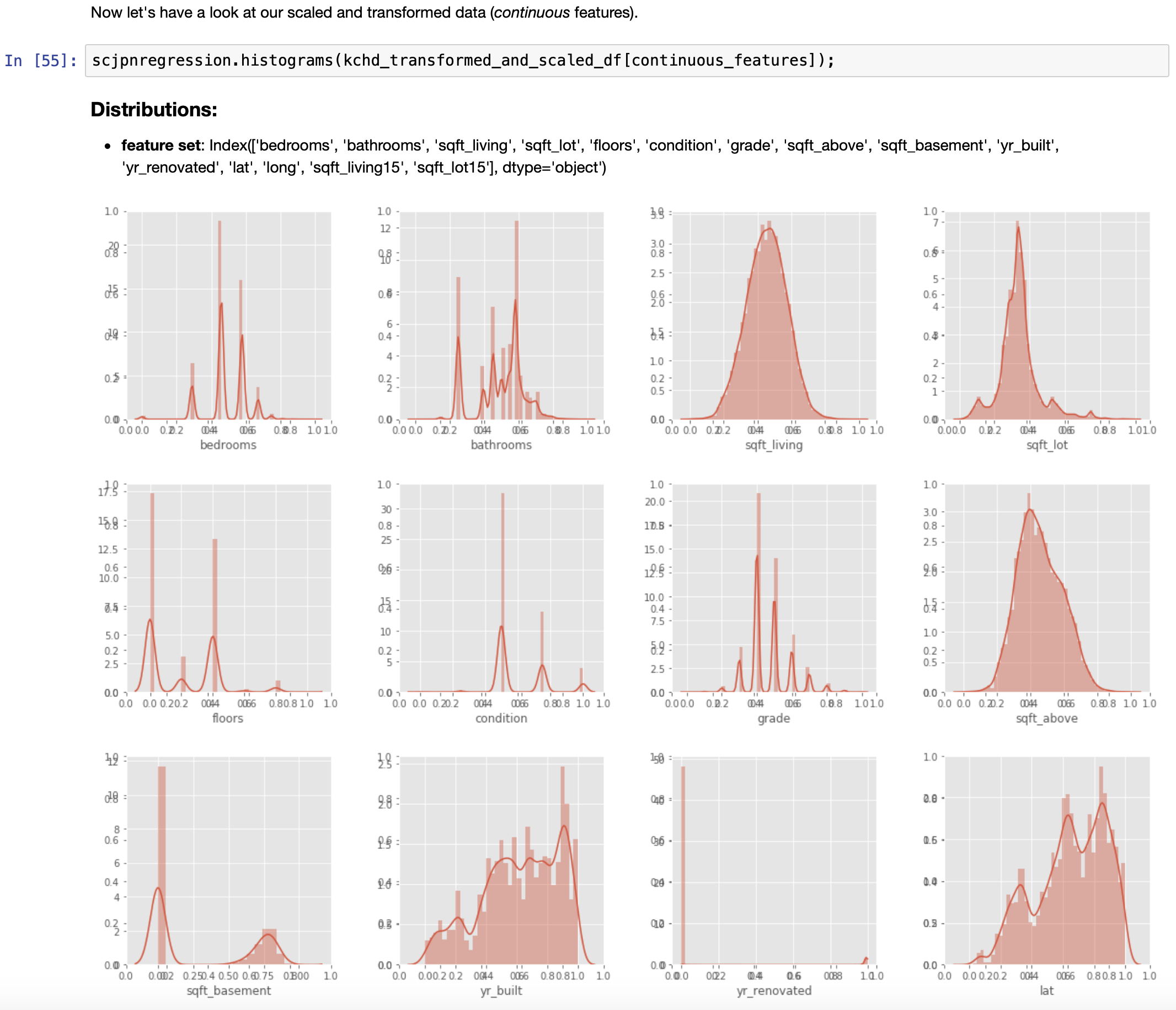
EDA, Round 2: Distributions and Linearity Study after scaling/transforming continuous predictors, as well as the response variable
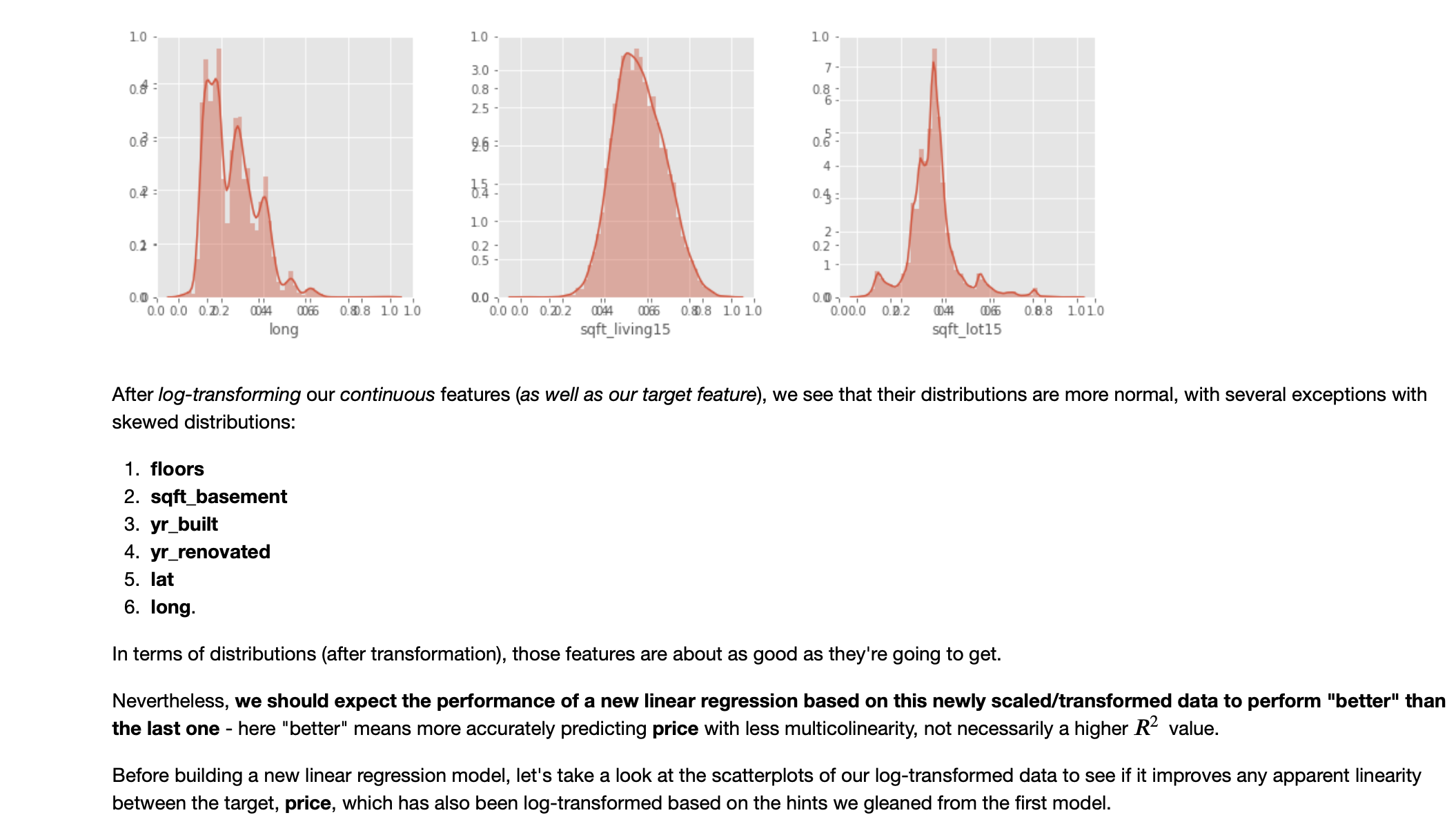
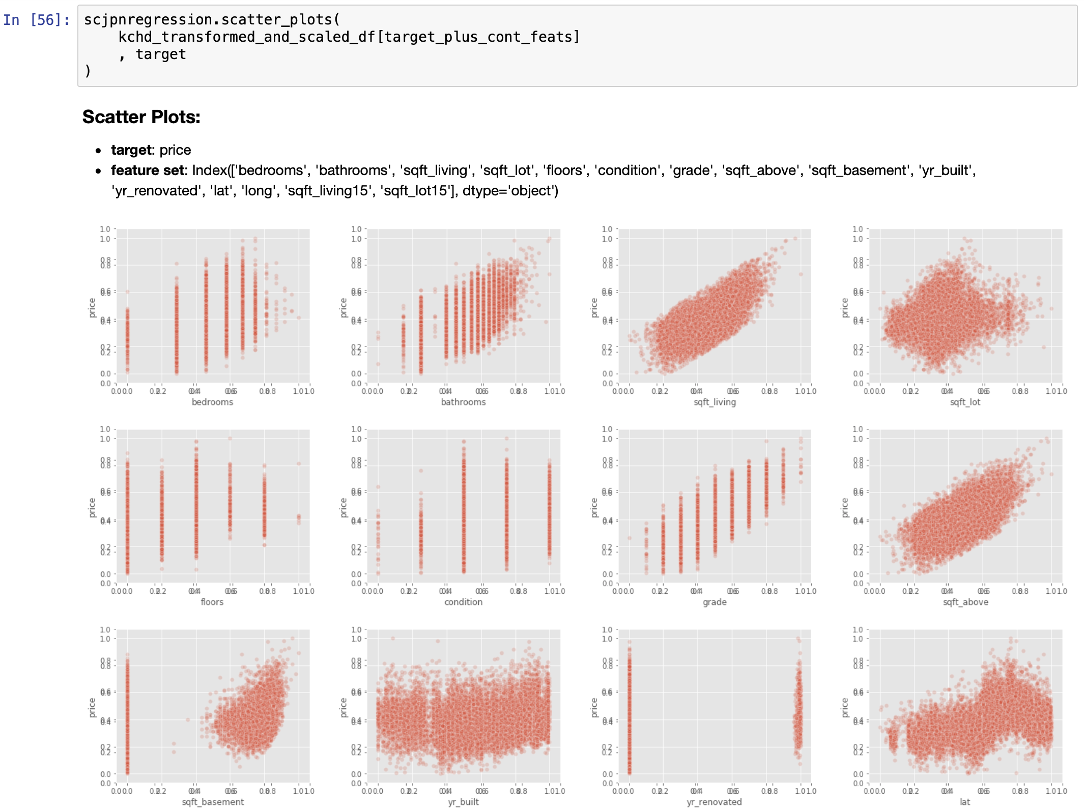

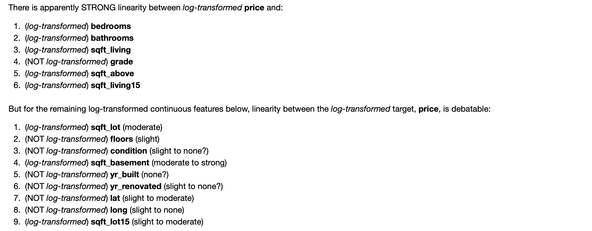
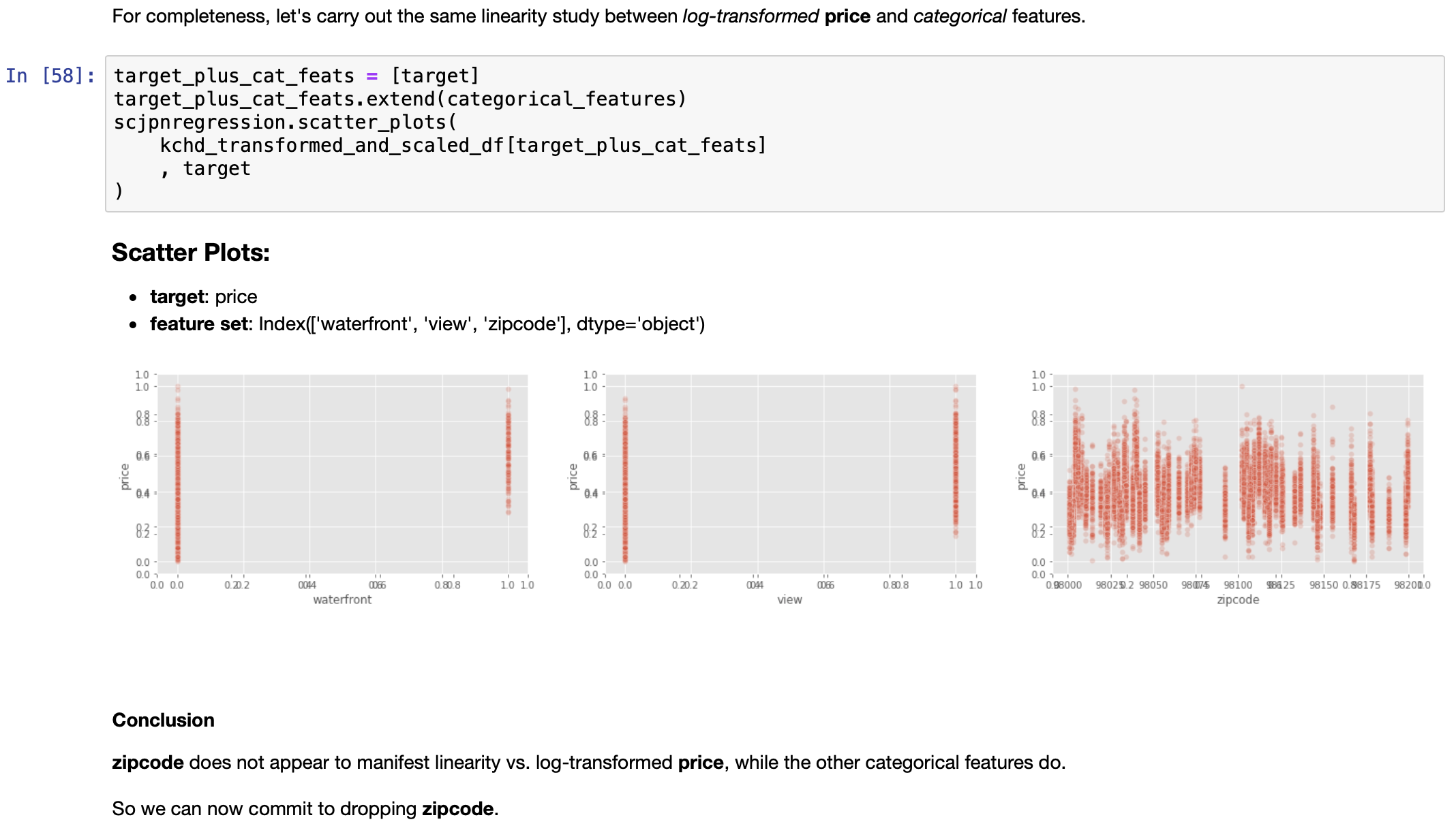
Iterative Refinement Continues

Note: output has been truncated in order to save space, therefore, I present only the resulting model comparison; for the full model output, please refer to the main notebook.
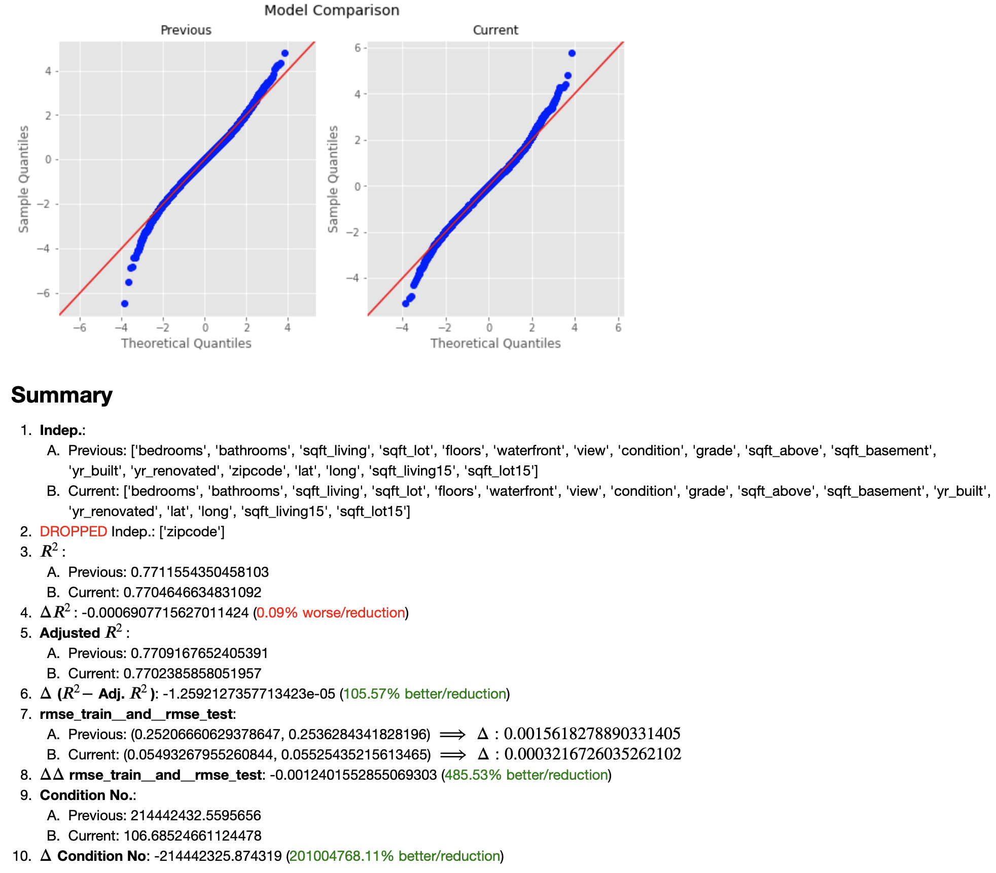
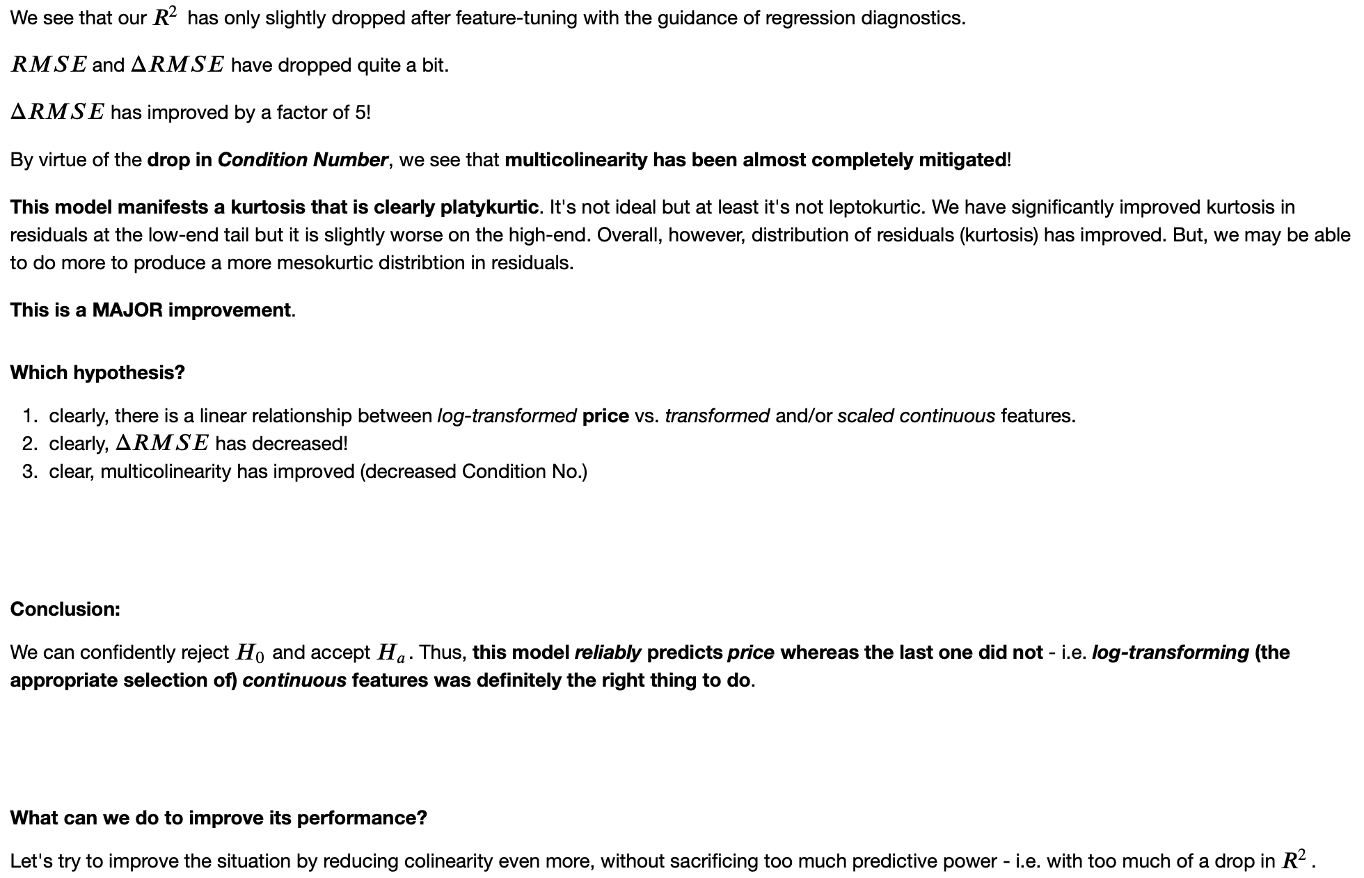
Note: from there, I follow this same pattern through a few more iterations in an attempt to vet out the features that are the most collinear; it involved examing correlation matrices and so forth but I will skip over that output since, as it turns out, that effort is largely unnecesary when we can simply rely on mathematics to tell us the answer; so, I will just skip forward to the juicy part but for a full treatment of iterative refinement, please have a look at the main notebook.
Submit Candidate-Feature Basis for Cross-Validation Forward Selection of Optimal Features

Note: for details on how this is done, please refer to the blog post I wrote about this topic.

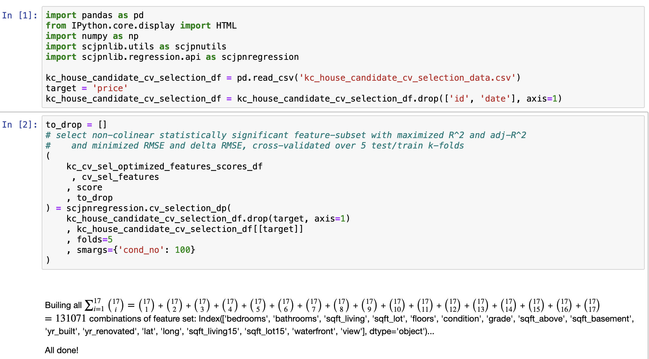
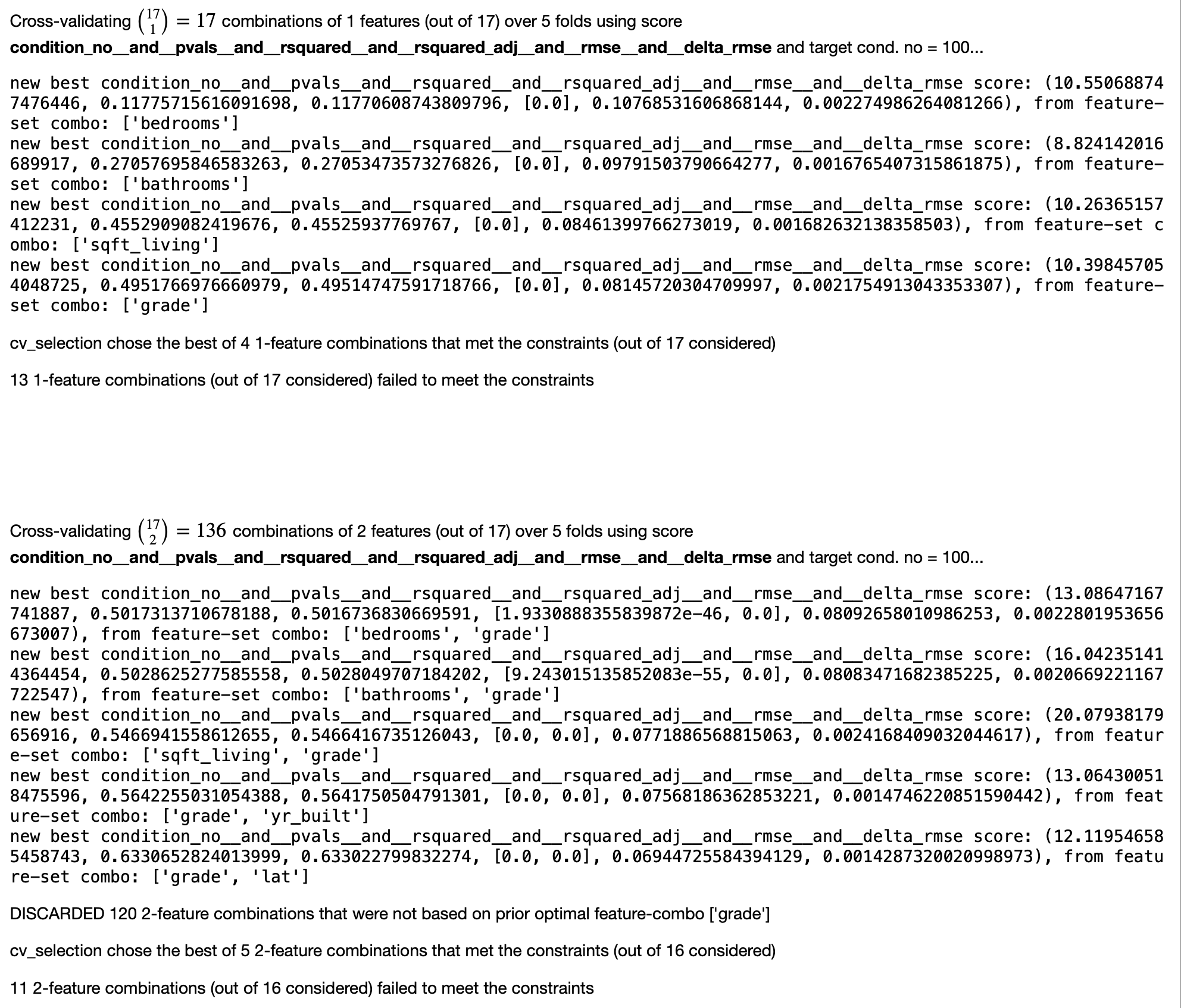
Note: output has been truncated in order to save space but from here but pattern is followed until it exhausts all available combinations that qualify; the end results is a list of feature subsets (of length \(k\)) that are optimal based on: max \(R^2\), minimized RMSE, and Condition No, \(\le 100\) (and therefore are considered minimally collinear); to see the full output, please see the separate Cross-Validation Forward Selection of Features notebook written specifically for this purpose.
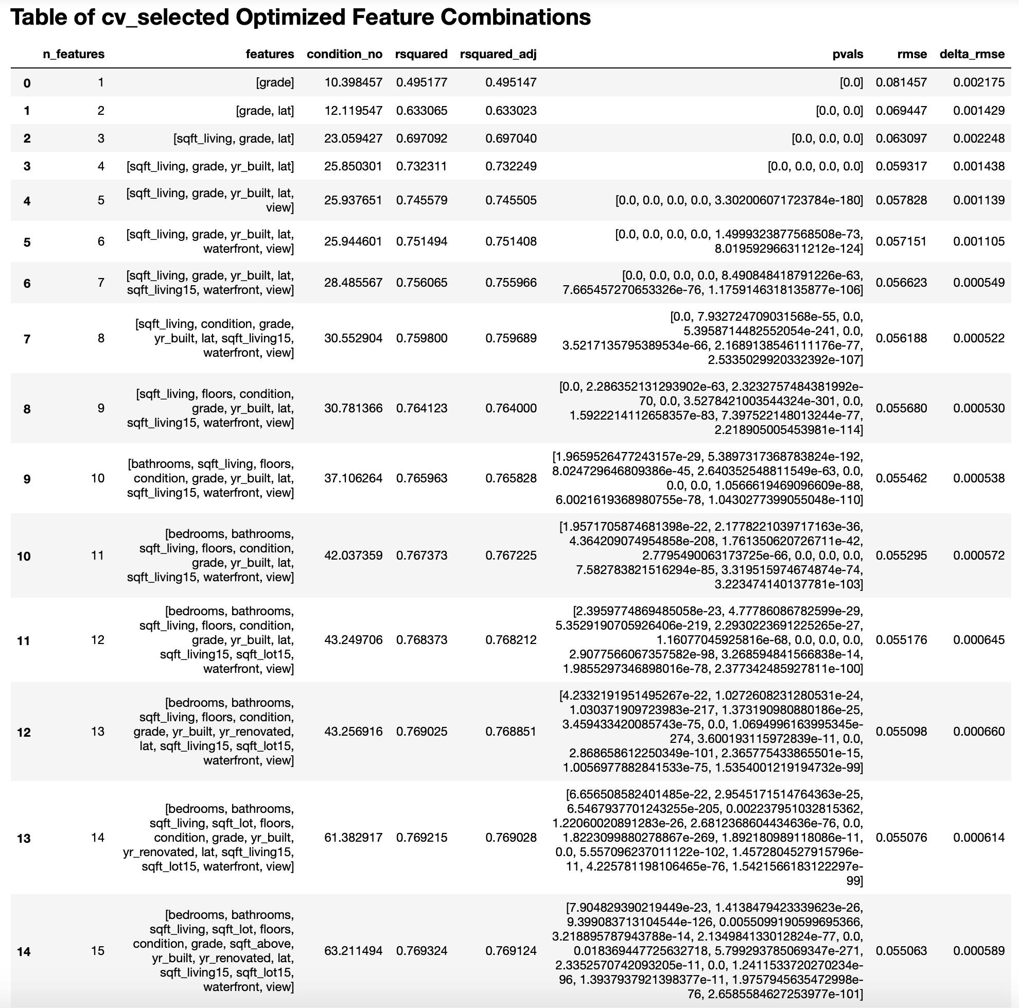
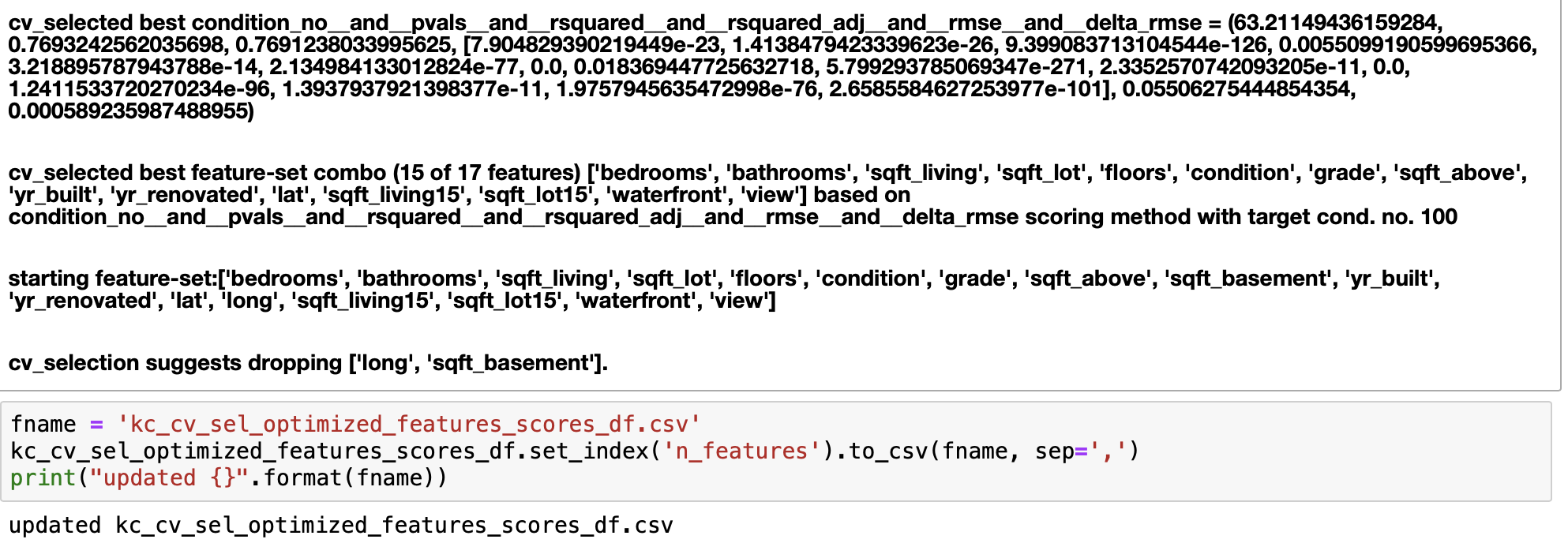
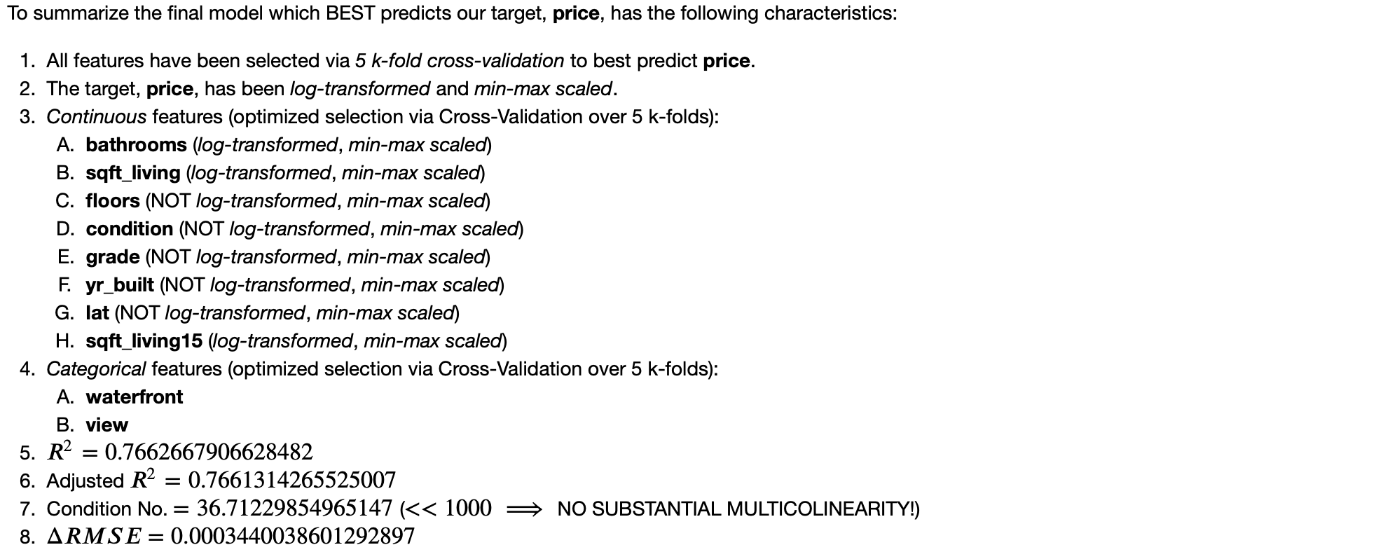
Skipping over some details that can be viewed in the main note book, we have the FINAL MODEL...

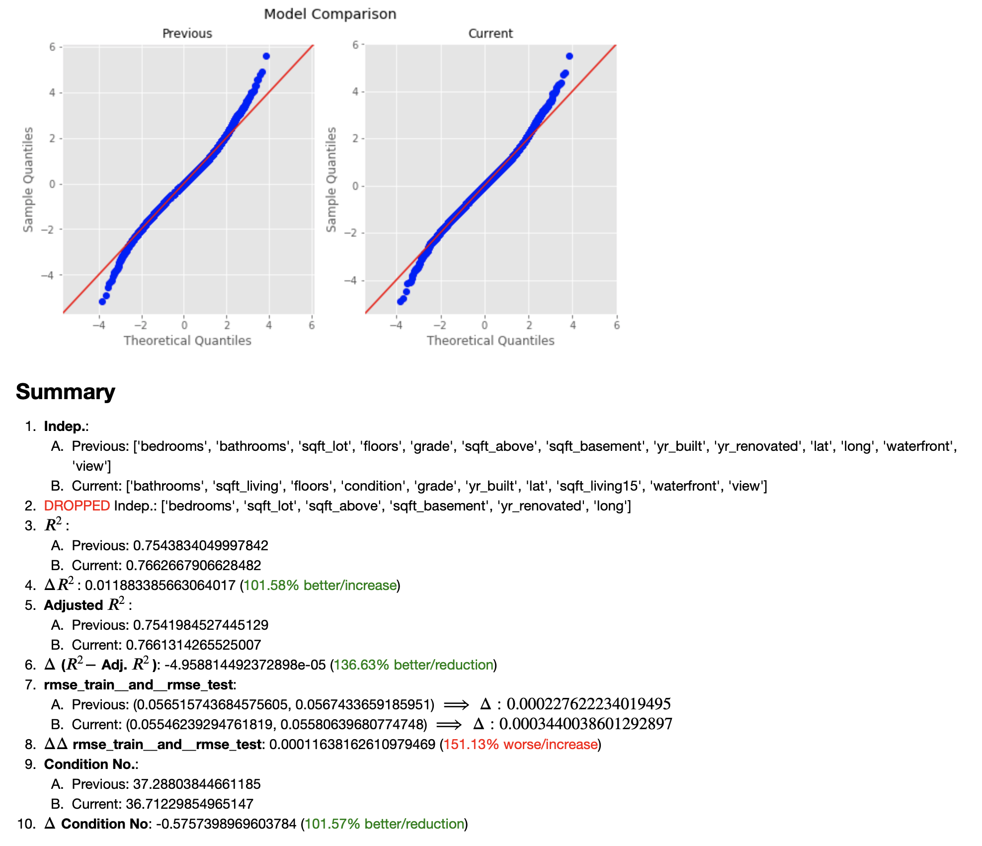
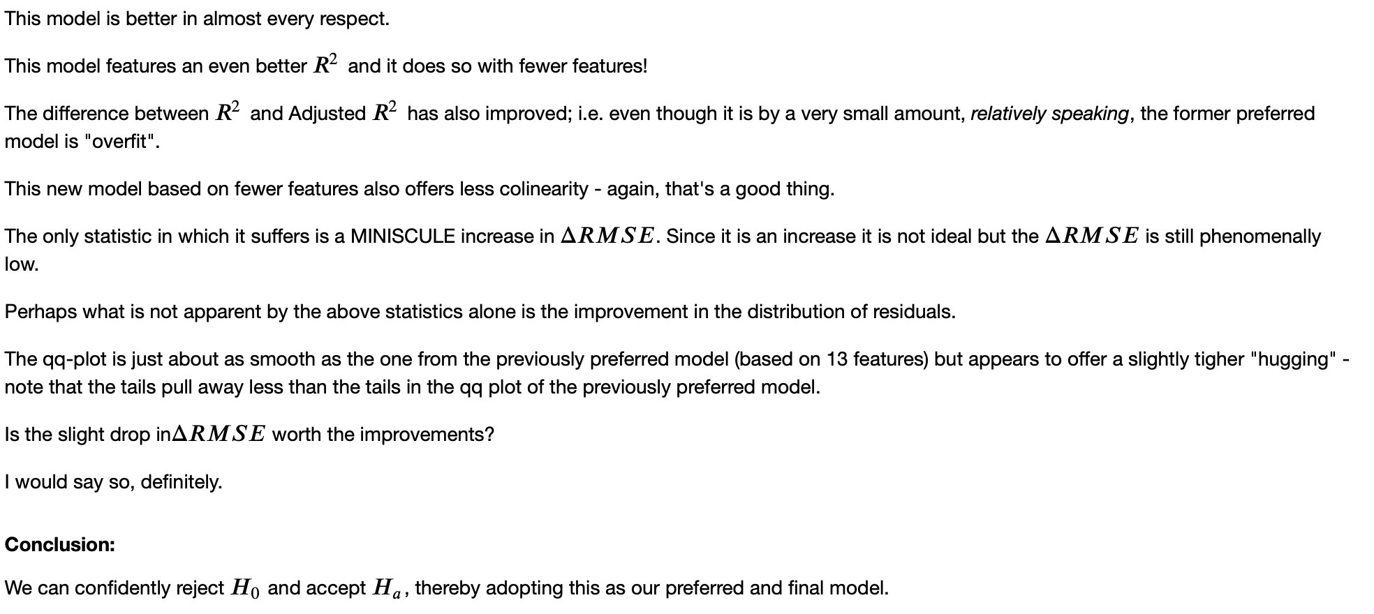
The FINAL Model
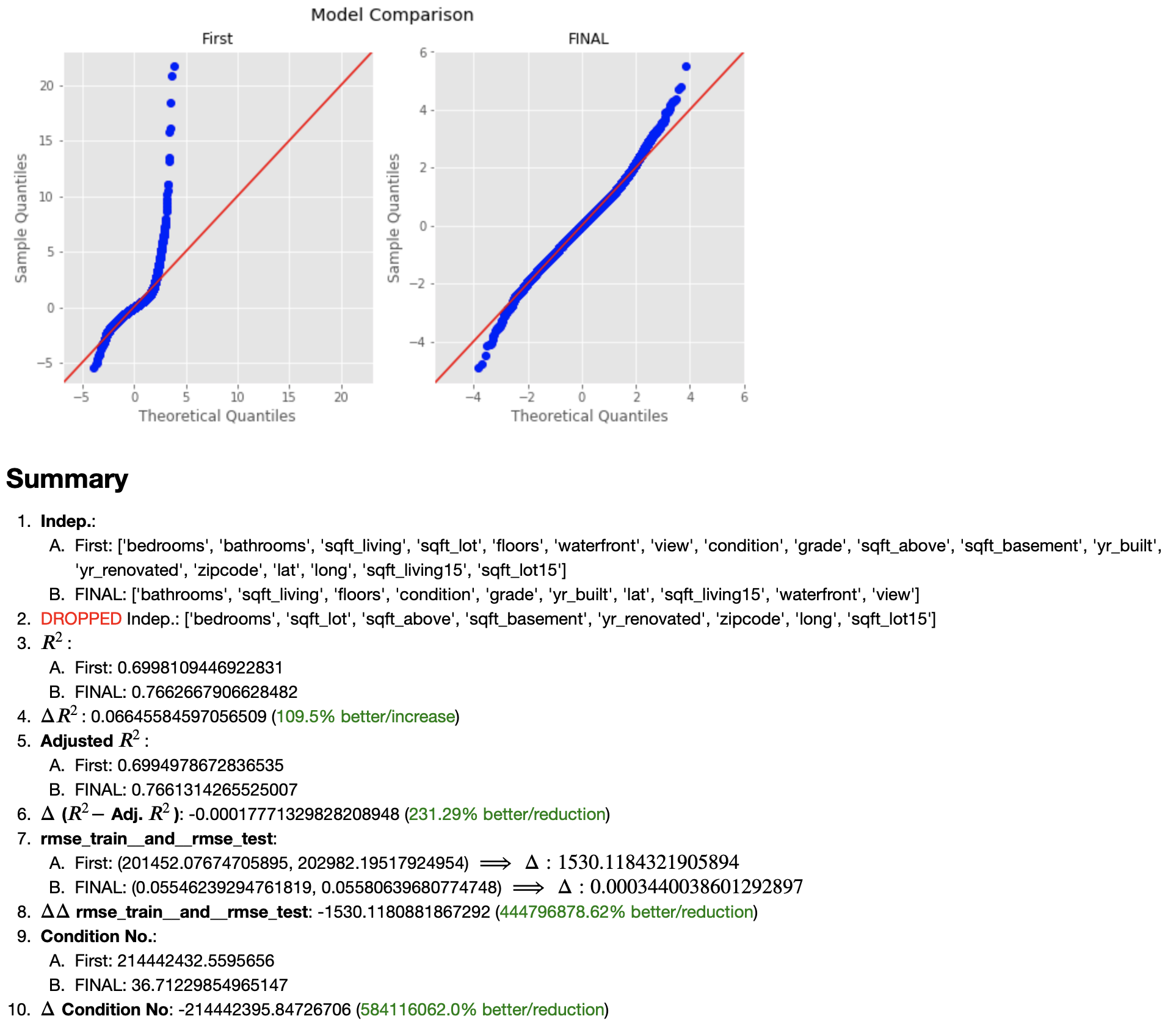
And how does it compare to the very first Preliminary Model?

Now we can finally move on to the most entertaining portion of the project: A "REAL WORLD" PROBLEM!
PUTTING THE FINAL MODEL TO USE: Solving a Real World Problem
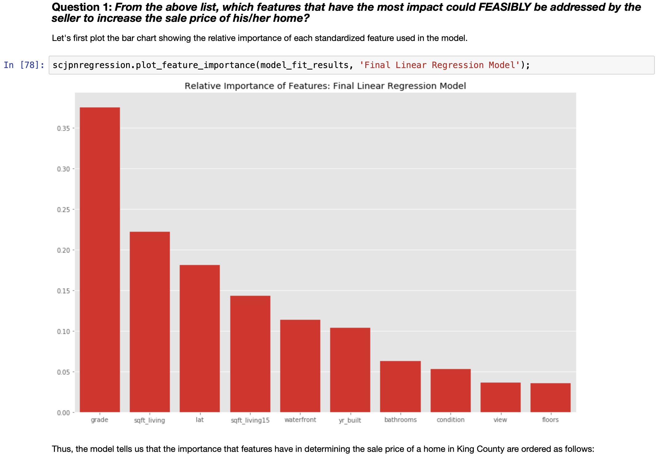
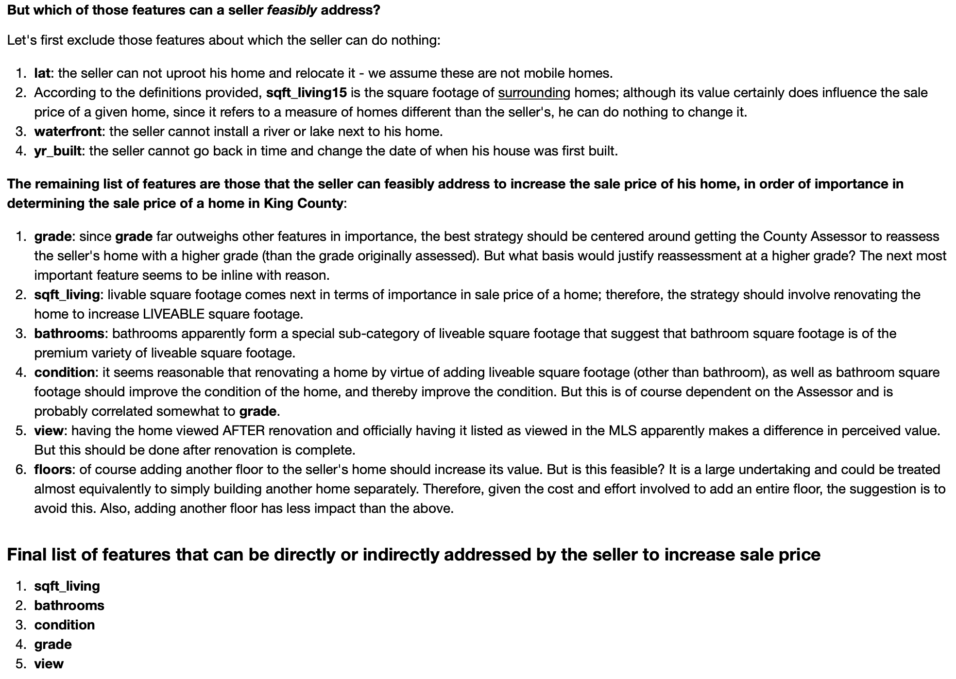

Let us see if the mathematics agrees.


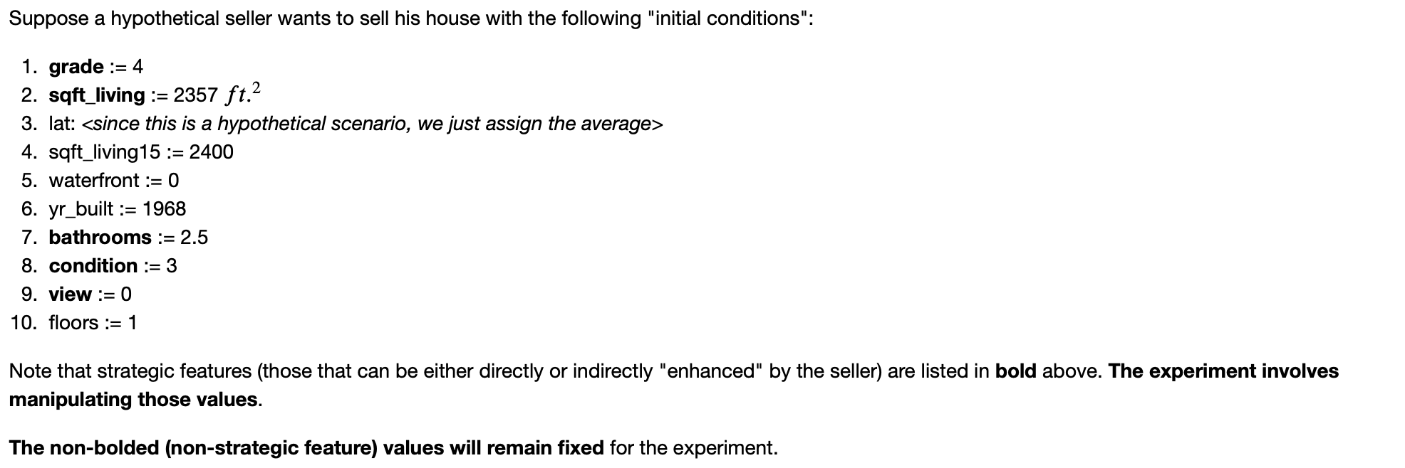

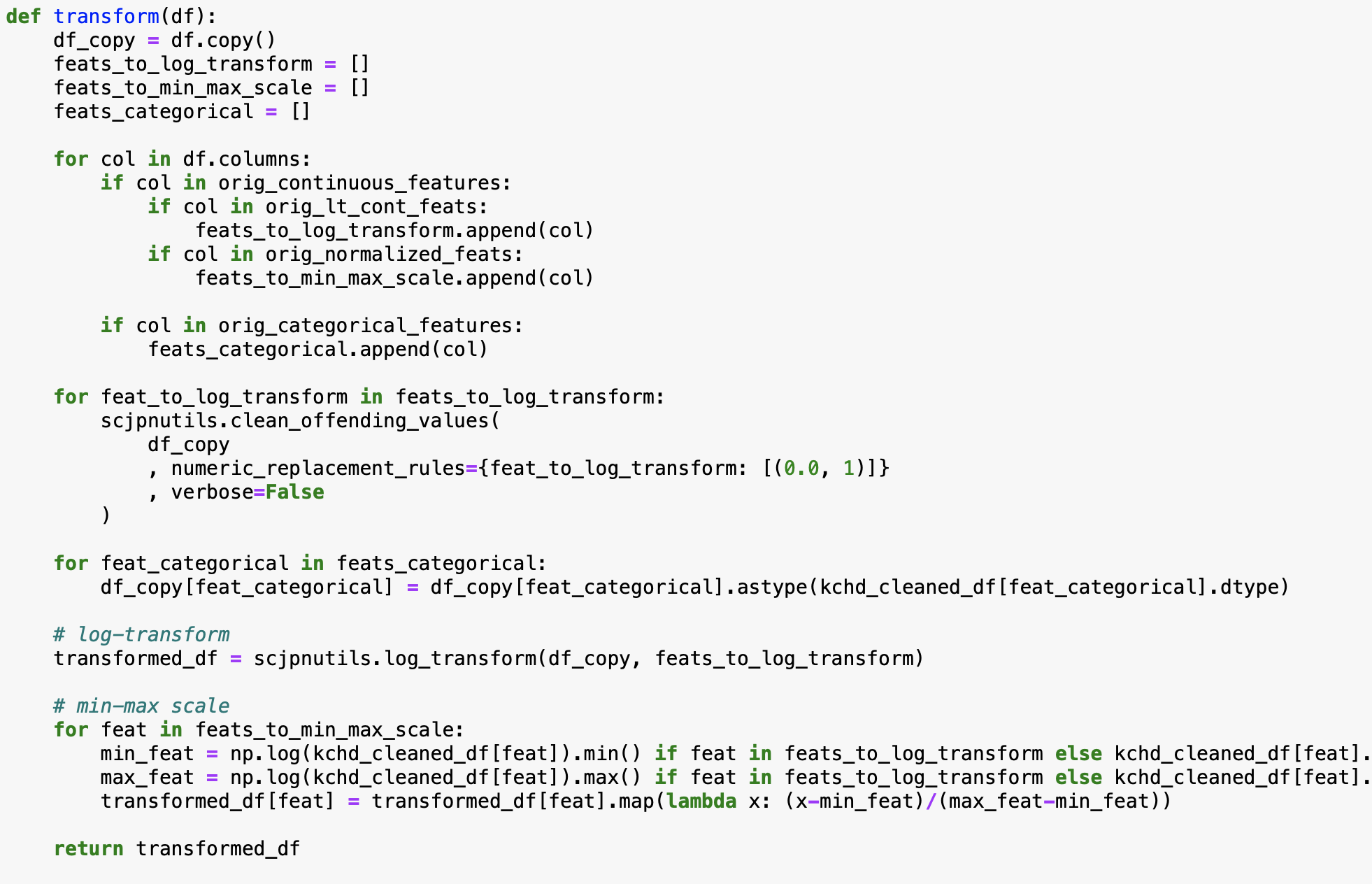
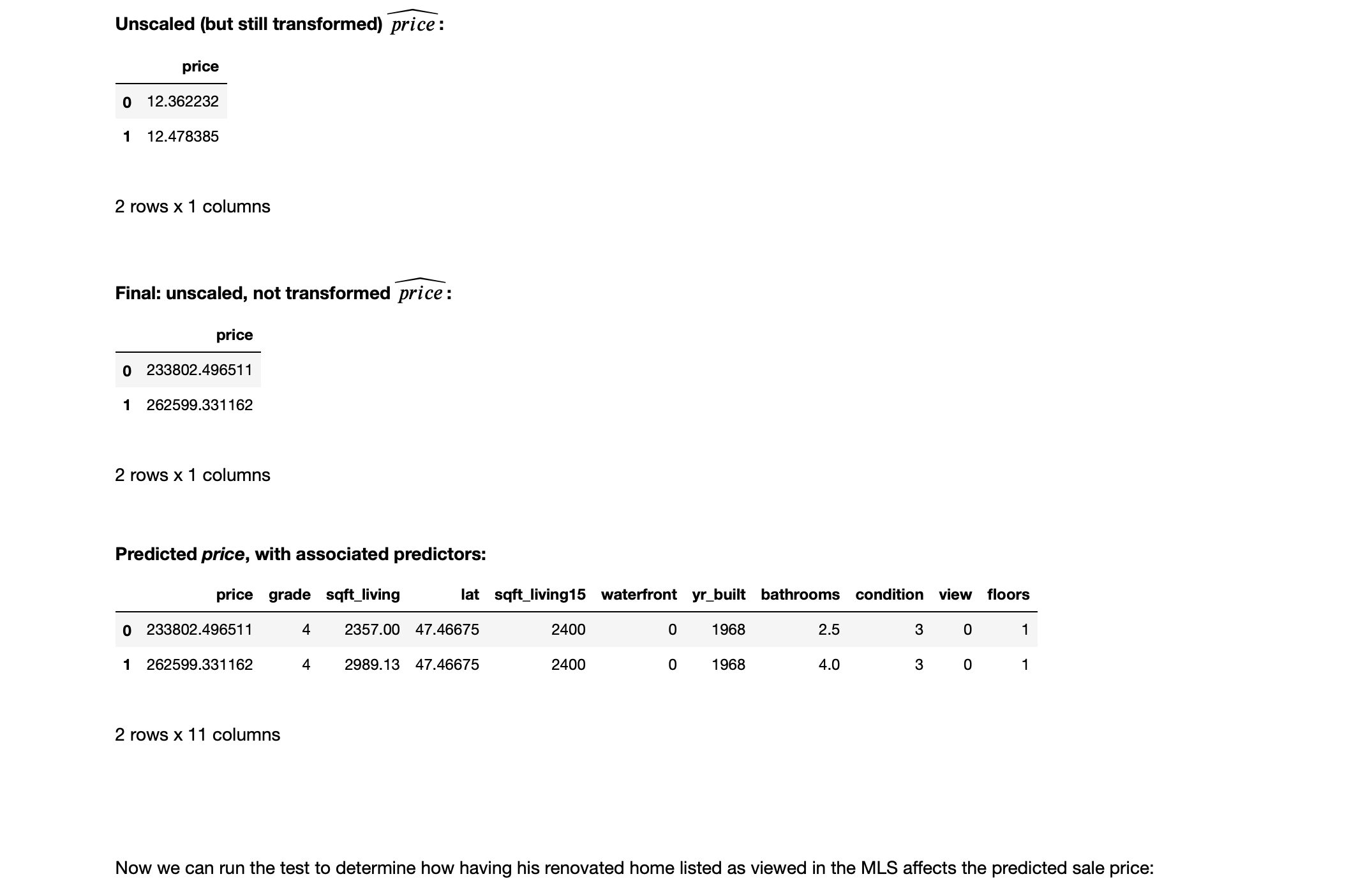
In order to answer this question, we must write a funtion to "undo" transformation and scaling (since that is how the values are stored in the dataframe).
The code below accomplishes this:
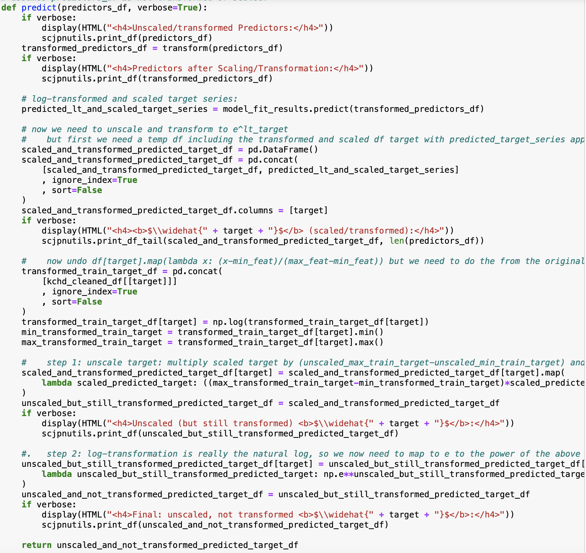
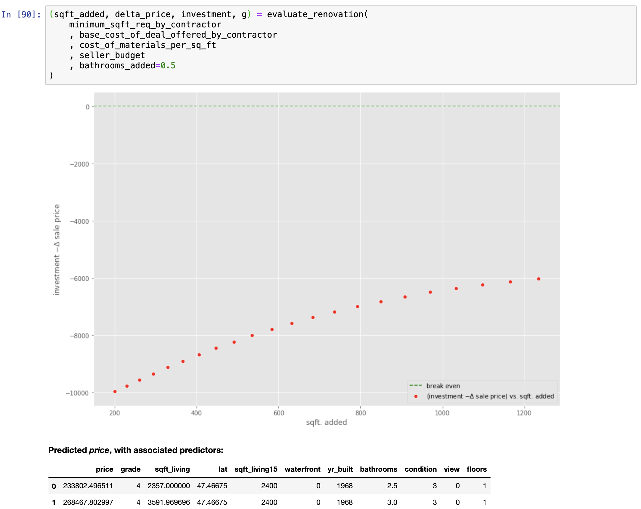
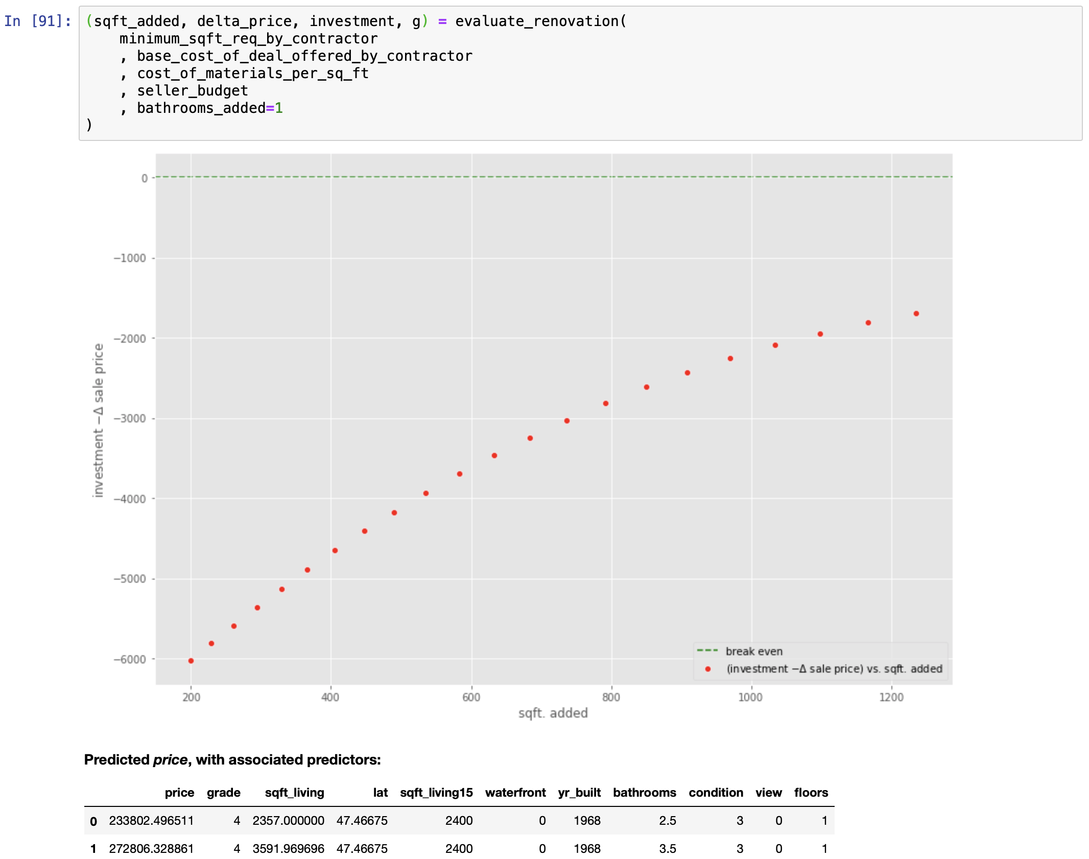
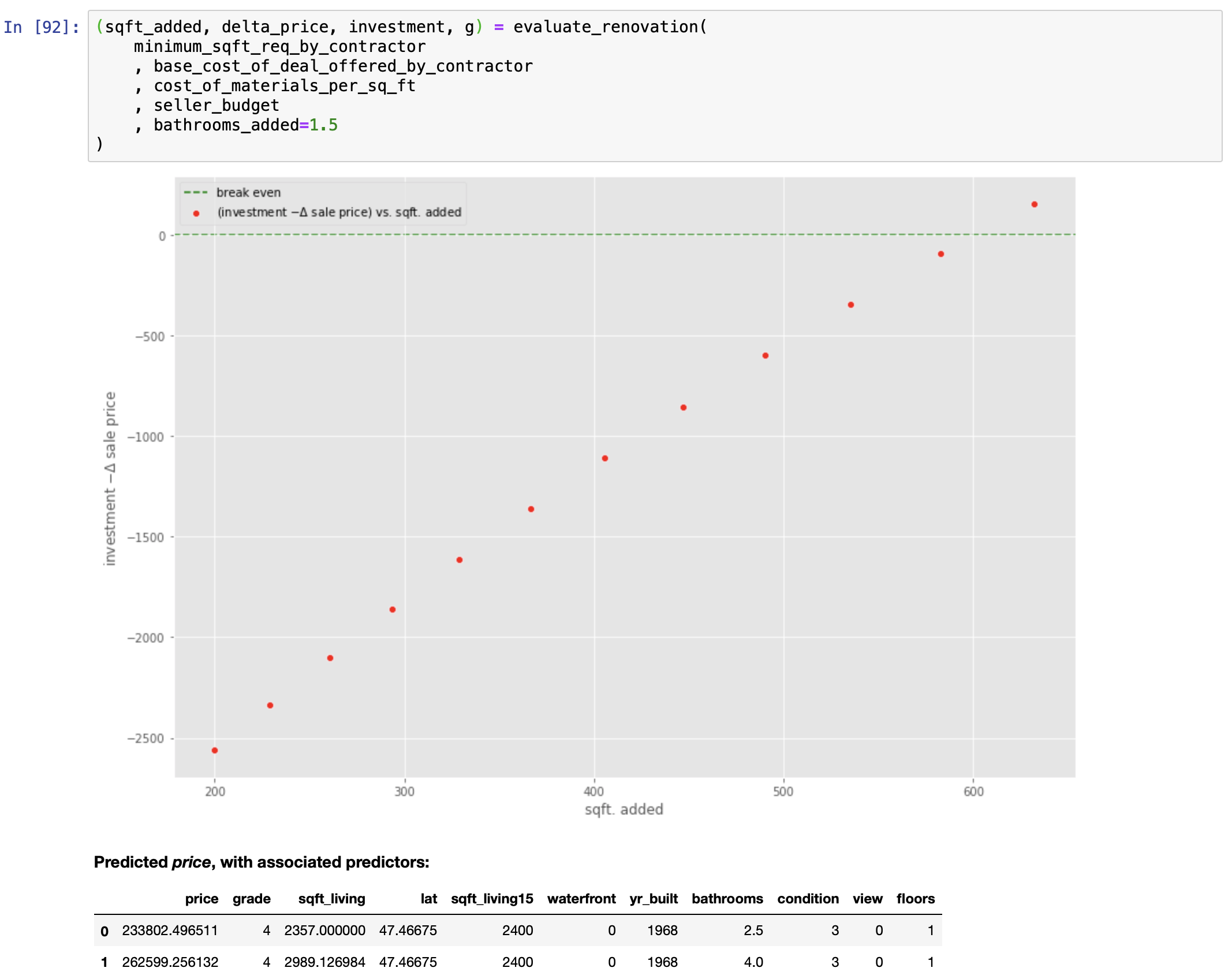
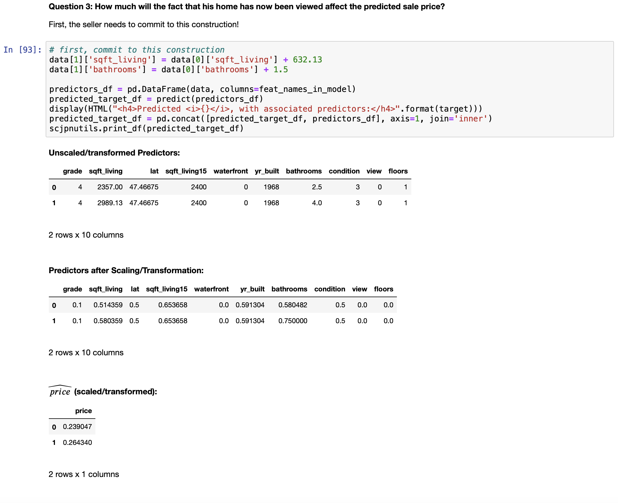
We can now answer this question:
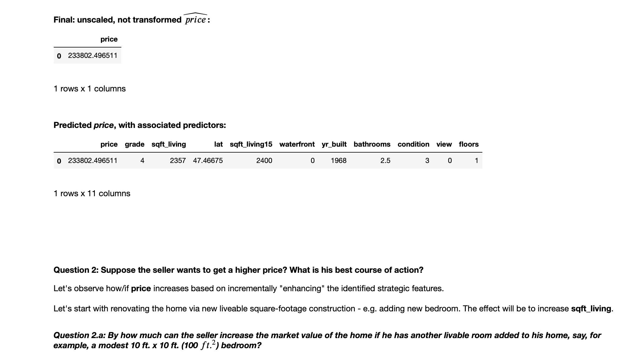
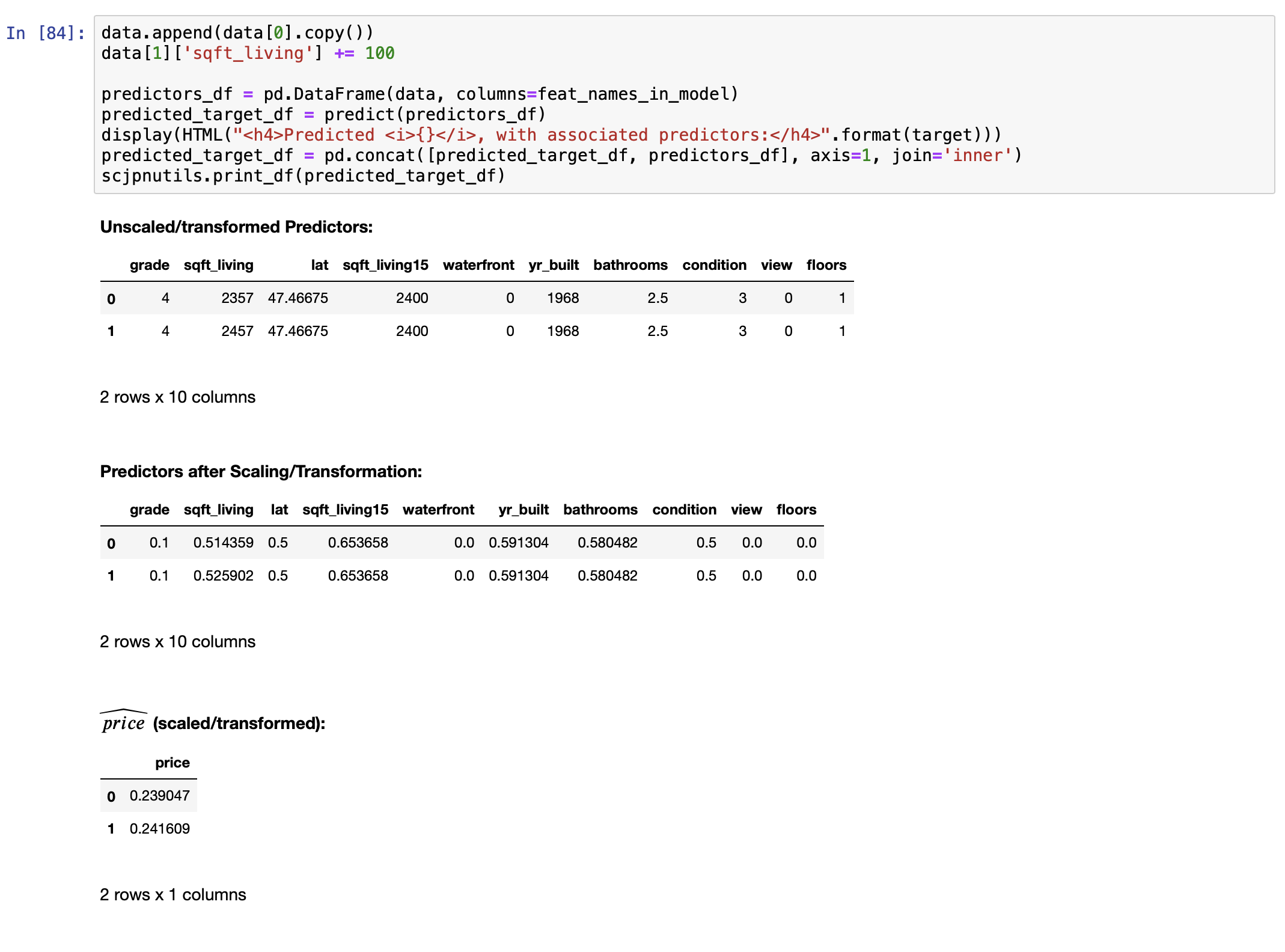
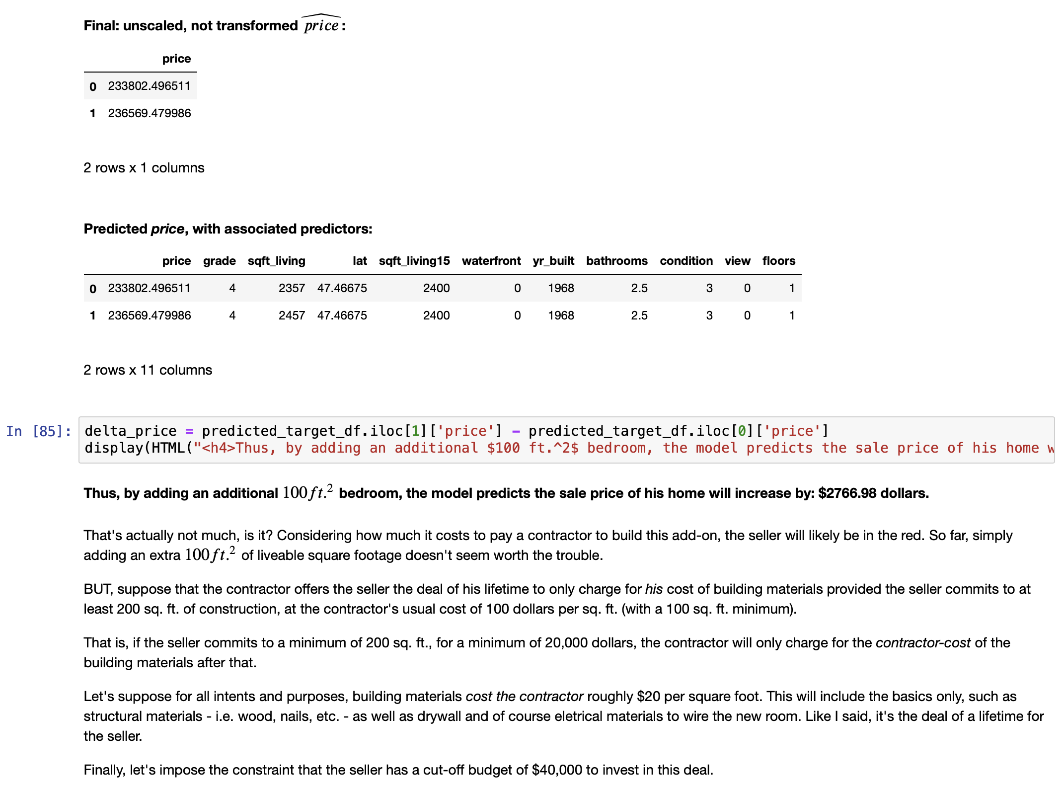

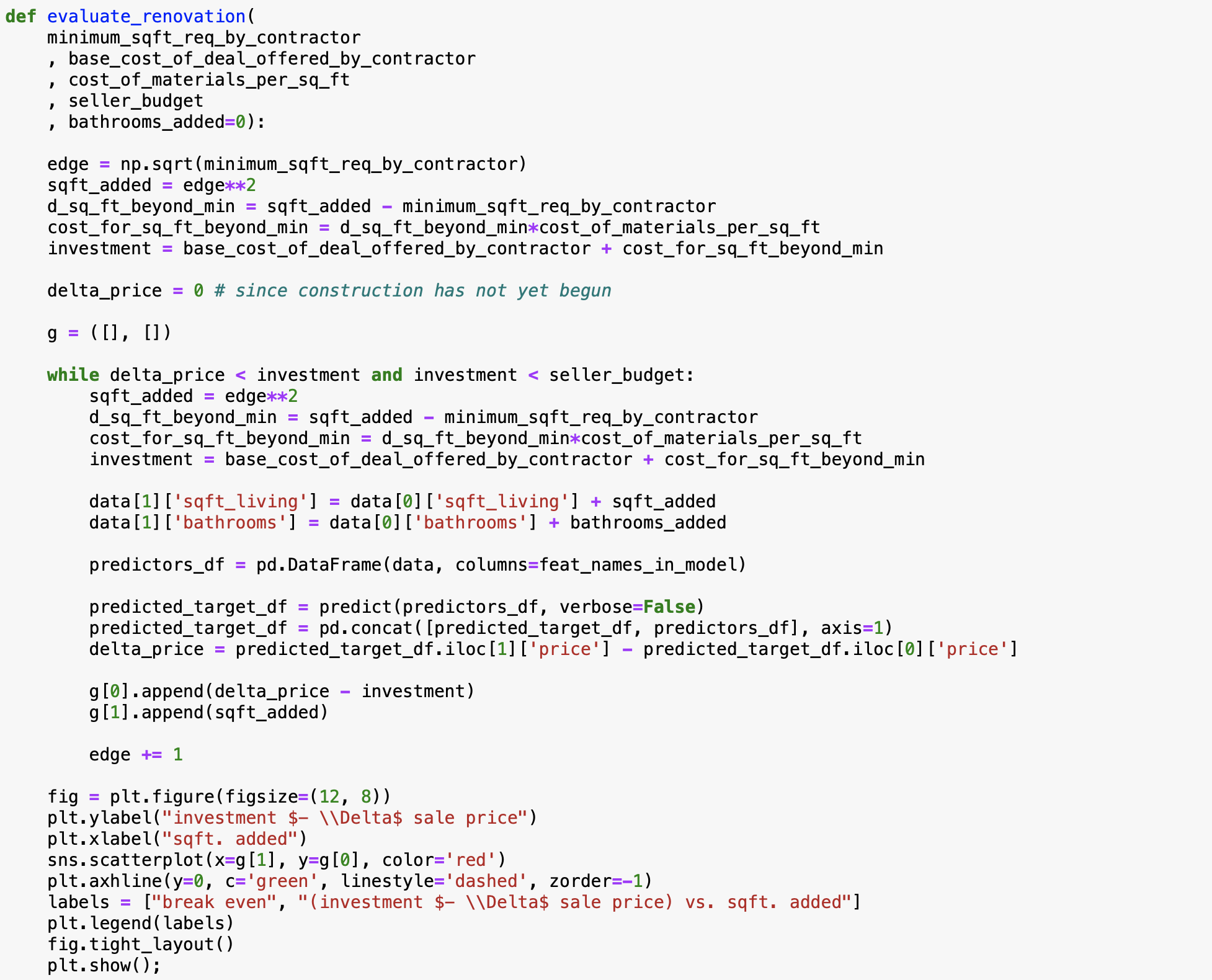
Answering this question requires the following special-purpose function:

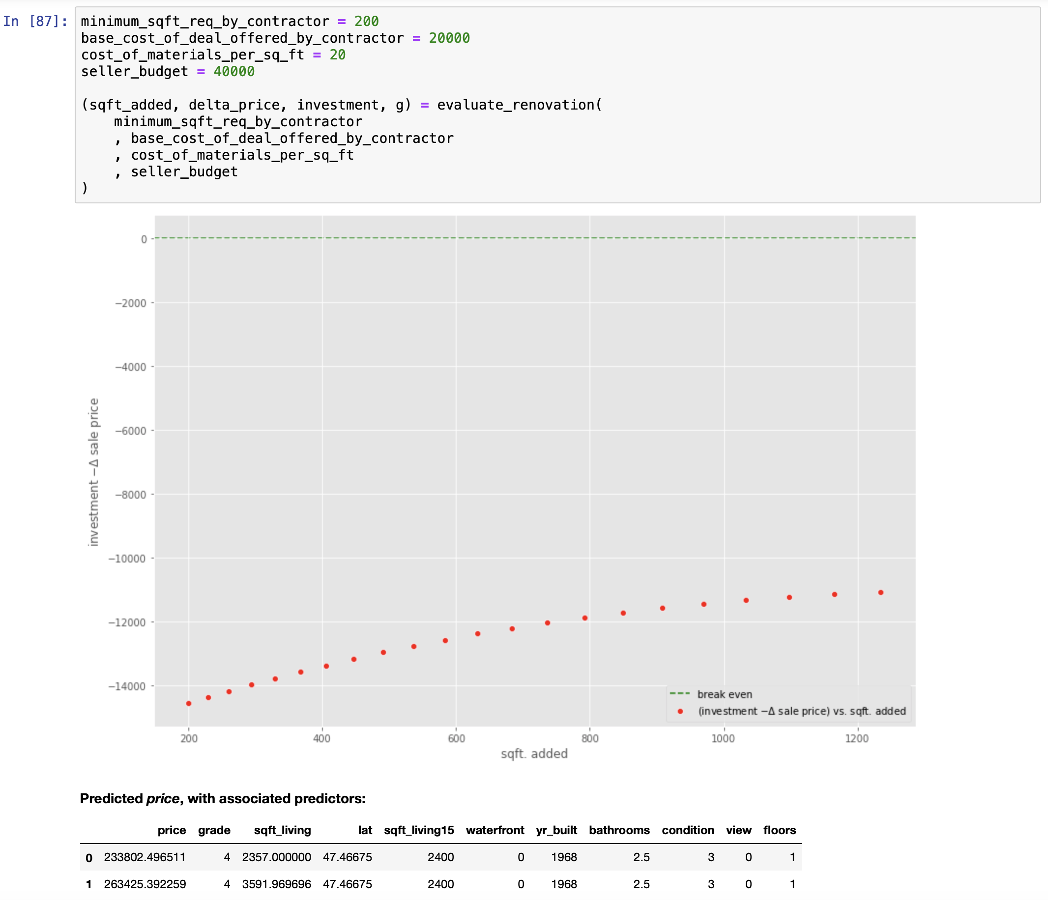
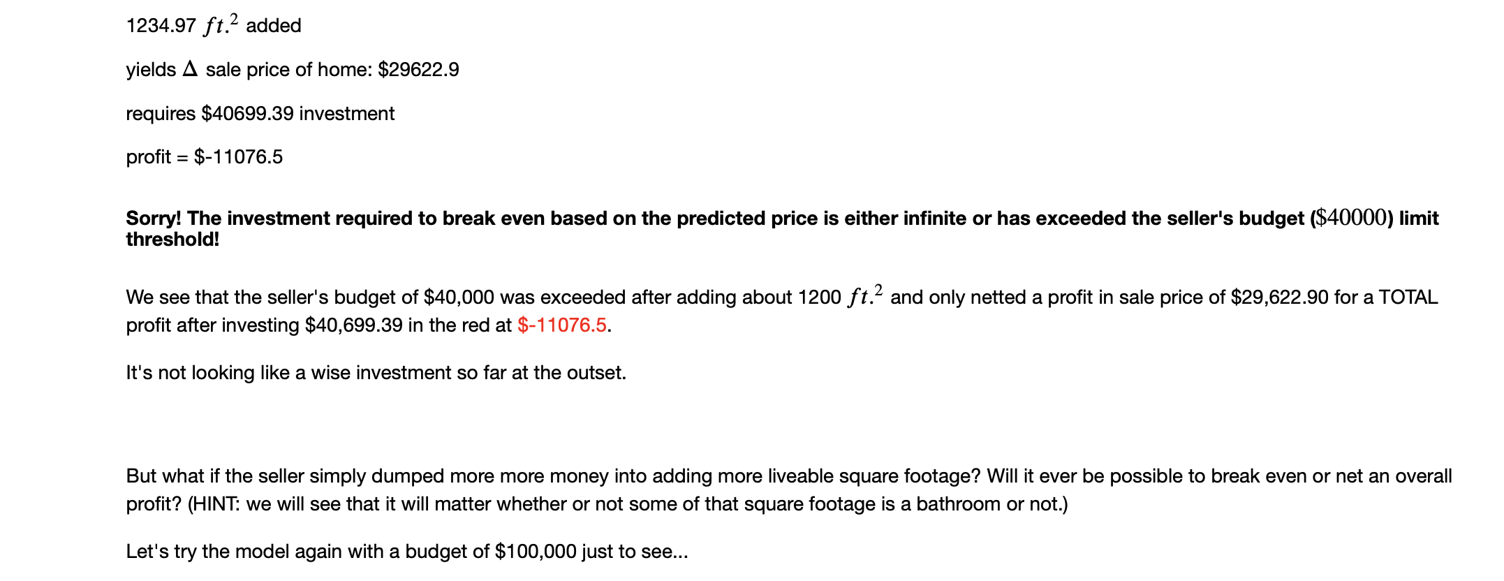
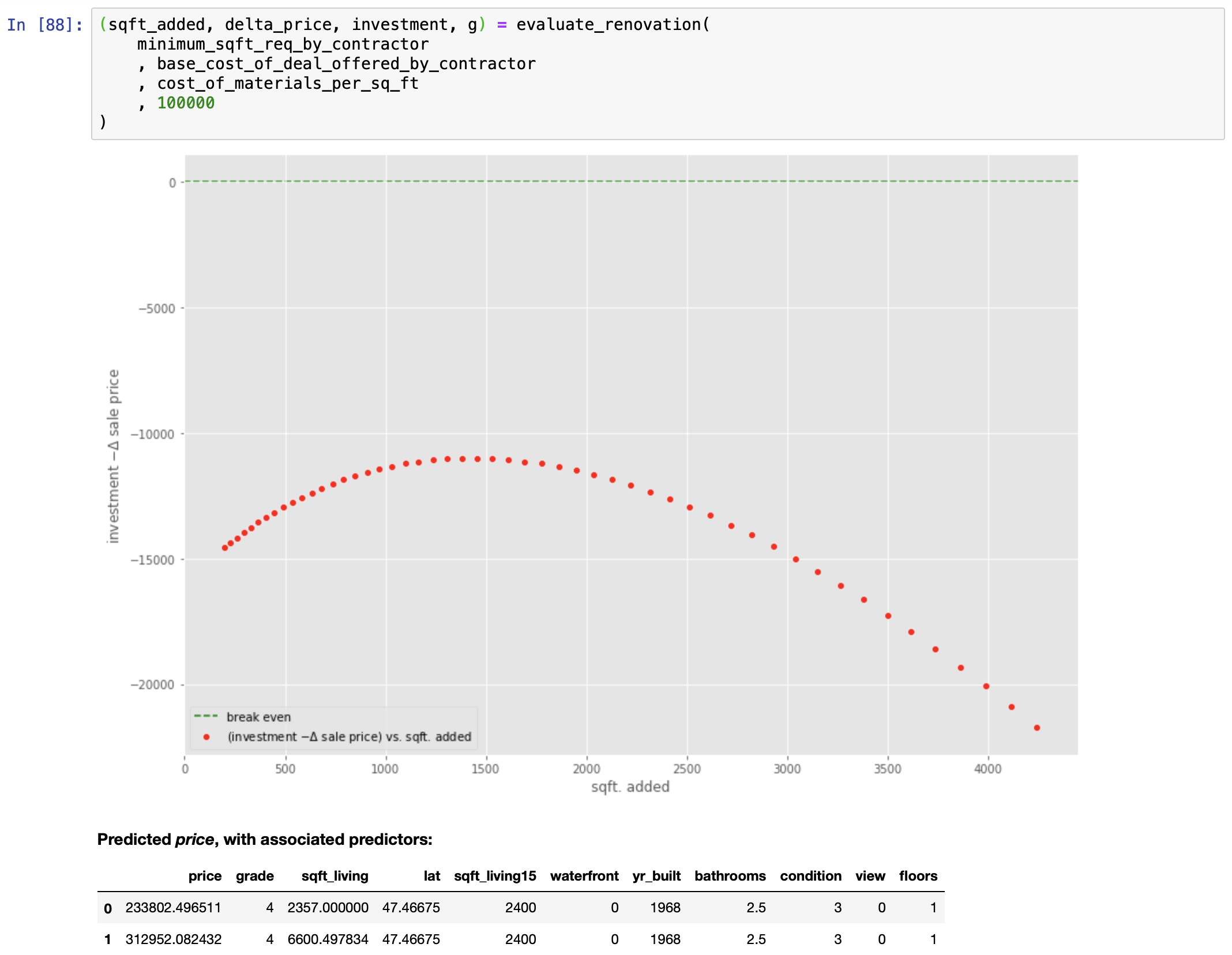
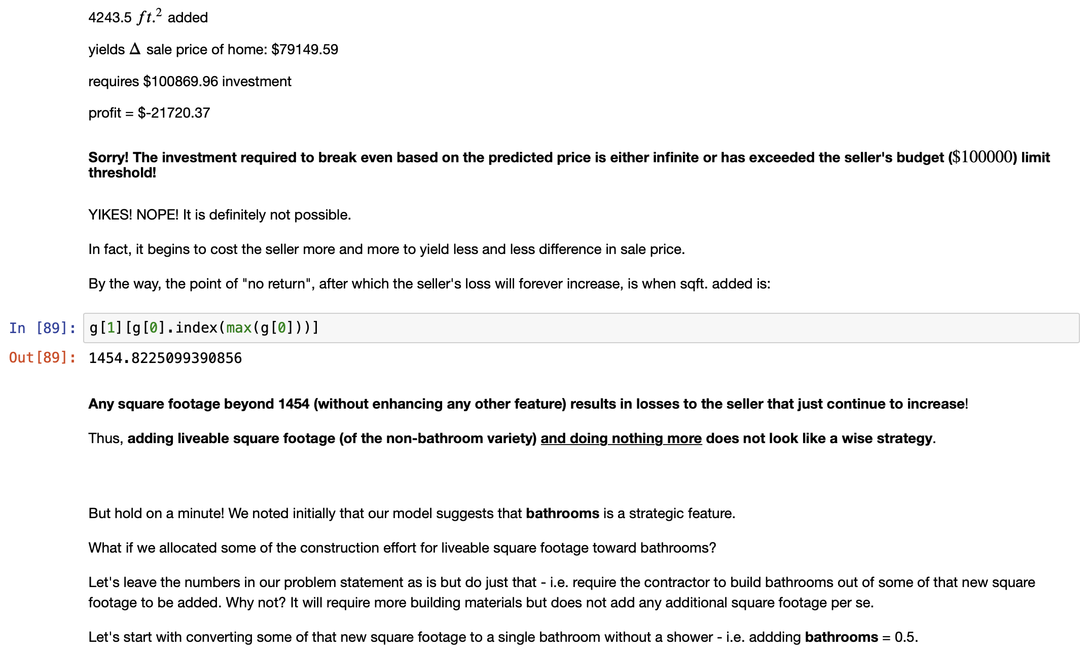




FIN
References
James, G., Witten, D., Hastie, T., & Tibshirani, R. (2012). An Introduction to Statistical Learning with Applications in R [Ebook] (7th ed.). New York, New York: Springer Science+Business Media. Retrieved from https://faculty.marshall.usc.edu/gareth-james/ISL/ISLR%20Seventh%20Printing.pdf
Lau, Dr. C. H. (2019). 5 Steps of a Data Science Project Lifecycle. Retrieved from https://towardsdatascience.com/5-steps-of-a-data-science-project-lifecycle-26c50372b492
Kurtosis. (2019). Retrieved from https://www.investopedia.com/terms/k/kurtosis.asp
Introduction to Mesokurtic. (2019). Retrieved from https://www.investopedia.com/terms/m/mesokurtic.asp
Understanding Leptokurtic Distributions. (2019). Retrieved from https://www.investopedia.com/terms/l/leptokurtic.asp
What Does Platykurtic Mean?. (2019). Retrieved from https://www.investopedia.com/terms/p/platykurtic.asp